Algorithmic Portfolio Optimization in Python
Author :: Kevin Vecmanis
In this installment I demonstrate the code and concepts required to build a Markowitz Optimal Portfolio in Python, including the calculation of the capital market line. I build flexible functions that can optimize portfolios for Sharpe ratio, maximum return, and minimal risk.
In this article you will learn:
- How to fetch stock market data from Quandl
- How to create a portfolio simulation function
- What the Markowitz Bullet is and how to plot one
- What the optimization process is all about
- What minimization functions are
- How to create an optimization function with scipy.optimize
- What the efficient frontier is and how to plot it
- What the capital market line is and how to plot it
Table of Contents
- Introduction
- Fetching data from Quandl
- Portfolio Simulation Function
- The Markowitz Bullet
- The Optimization Process
- Minimization Functions
- The Optimization Function
- The Efficient Frontier
- The Capital Market Line
Introduction
Portfolio optimization is a mathematically intensive process that can be accomplished with a variety of optimization functions that are freely available in Python.
In Part 1 of this series, we’re going to accomplish the following:
- Build a function to fetch asset data from Quandl.
- Show how this data can be converted into return matrix and a covariance matrix.
- Show how to simulate a basket of thousand of portfolios using the same assets.
- Show how portfolio weights can be optimized for either volatility, returns, or Sharp Ratio.
- Build the Markowitz efficient frontier.
- Build the Capital market line.
- Calculatet the optimal portfolio weights based on the intersection of the capital market line with the efficient frontier.
The theory behind the capital market line and efficient frontier is outside the scope of this post, but plenty of material is available with a quick google search on the topic. Explanations of concepts will be provided throughout this post as required. I assume here that the reader has a basic familiarity with modern portfolio theory (MPT).
Fetching data from Quandl
The first function we define pulls assets from Quandl based on a list of ticker names that we provide in the variable ‘assets’.
# Standard Python library imports
import pandas as pd

# 3rd party imports
import quandl

def fetch_data(assets):

    '''
    Parameters:
    -----------
        assets: list
            takes in a range of ticker symbols to be pulled from Quandl.
            Note: It's imporant to make the data retrieval flexible to multiple assets because
            we will likely want to back-test strategies based on cross-asset technical
            indictors are ratios!  It's always a good idea to put the work and thought
            in upfront so that your functions are as useful as possible.

    Returns:
    --------
        df: Dataframe
            merged market data from Quandl using the date as the primary merge key.
    '''

    count = 0
    auth_tok = '<your Quandl key>'

    #instatiate an empty dataframe
    df = pd.DataFrame()

    # Because we will potentially be merging multiple tickers, we want to rename
    # all of the income column names so that they can be identified by their ticker name.
    for asset in assets:
        if (count == 0):
            df = quandl.get('EOD/' + asset, authtoken = auth_tok)
            column_names=list(df)

            for i in range(len(column_names)):
                column_names[i] = asset + '_' + column_names[i]
            df.columns = column_names
            count += 1
        else:
            temp = quandl.get('EOD/' + asset, authtoken = auth_tok)
            column_names = list(temp)

            for i in range(len(column_names)):
                column_names[i] = asset+'_' + column_names[i]

            temp.columns = column_names
            # Merge all the dataframes into one with new column names
            df = pd.merge(df, temp, how = 'outer', left_index = True, right_index = True)

    return df.dropna(inplace = True)
We’re going to complete this post by optimizing portfolio weights for a basket of five assets:
TLT: Long bond ETF
GLD: Gold
SPY: S&P 500 ETF
QQQ: Nasdaq ETF
VWO: Emerging Market ETF
data = fetch_data (['TLT','GLD','SPY','QQQ','VWO'])Quandl data comes with a bunch of different column headers - but here we will strip out only the adjusted closes of each asset by creating a mask.
features = [f for f in list(df) if "Adj_Close" in f]
print(features)
['TLT_Adj_Close', 'GLD_Adj_Close', 'SPY_Adj_Close', 'QQQ_Adj_Close', 'VWO_Adj_Close']
adj_closes = df[features]
list(adj_closes)
Now our dataframe will only contain columns with the adjusted closes listed above.
By plotting the normalized adjusted closes we can see the relative performance of each asset. The ideal portfolio will benefit from assets that tend to covary in opposing ways.
import matplotlib.pyplot as plt
(adj_closes/adj_closes.iloc[0]*100).plot(figsize=(18,14))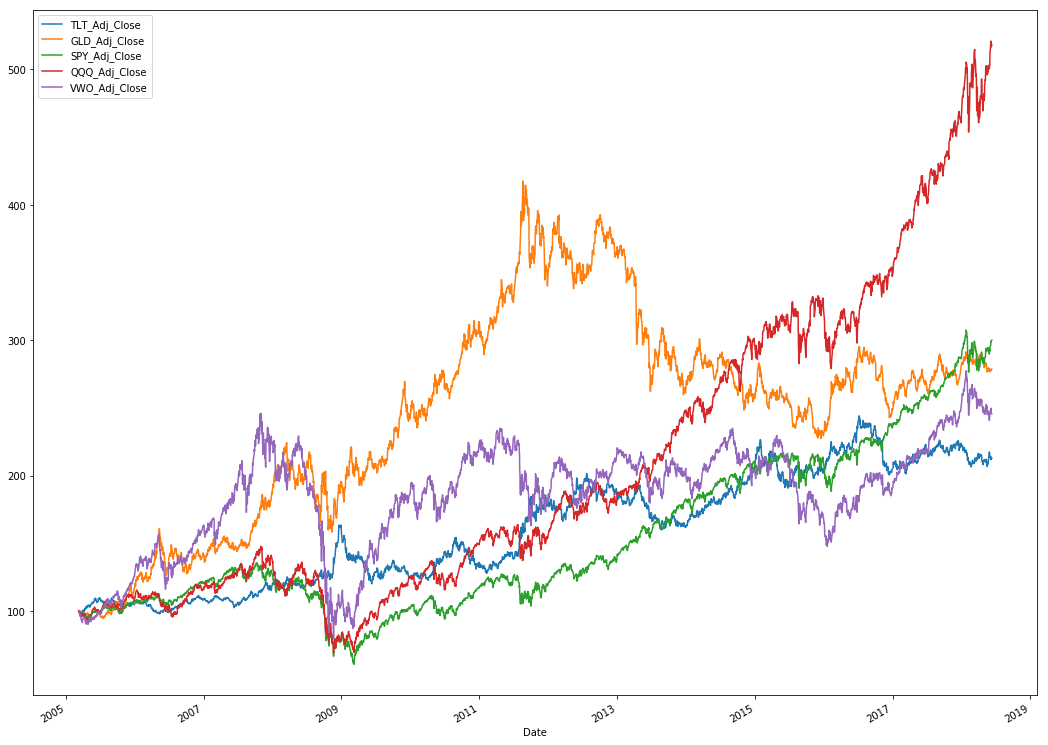
Next we can calculate the daily average returns for each asset in the dataset by doing the following
import numpy as np
returns = np.log(adj_closes/adj_closes.shift(1))
returns.mean()
TLT_Adj_Close 0.000226
GLD_Adj_Close 0.000307
SPY_Adj_Close 0.000329
QQQ_Adj_Close 0.000493
VWO_Adj_Close 0.000269
dtype: float64
To get the average annualized returns we multiple by 252 trading days
returns.mean() * 252TLT_Adj_Close 0.057061
GLD_Adj_Close 0.077453
SPY_Adj_Close 0.083012
QQQ_Adj_Close 0.124264
VWO_Adj_Close 0.067879
dtype: float64
returns.cov() TLT_Adj_Close GLD_Adj_Close SPY_Adj_Close QQQ_Adj_Close VWO_Adj_Close
TLT_Adj_Close 0.000076 0.000012 -0.000043 -0.000042 -0.000057
GLD_Adj_Close 0.000012 0.000142 0.000005 0.000001 0.000037
SPY_Adj_Close -0.000043 0.000005 0.000141 0.000137 0.000189
QQQ_Adj_Close -0.000042 0.000001 0.000137 0.000161 0.000188
VWO_Adj_Close -0.000057 0.000037 0.000189 0.000188 0.000339
Likewise, we can get the annualized covariance matrix for these 5 assets accordingly
returns.cov() * 252 TLT_Adj_Close GLD_Adj_Close SPY_Adj_Close QQQ_Adj_Close VWO_Adj_Close
TLT_Adj_Close 0.019235 0.003047 -0.010901 -0.010618 -0.014447
GLD_Adj_Close 0.003047 0.035806 0.001322 0.000274 0.009242
SPY_Adj_Close -0.010901 0.001322 0.035492 0.034597 0.047544
QQQ_Adj_Close -0.010618 0.000274 0.034597 0.040468 0.047254
VWO_Adj_Close -0.014447 0.009242 0.047544 0.047254 0.085304
The following single line of code generates a random array of weights that sum to 1.0. In the portfolio, one of the assumptions is that all funds will deployed to the assets in the portfolio according to some weighting.
weights = np.random.dirichlet(np.ones(num_assets), size=1)
weights = weights[0]
print(weights)
[0.1158917 0.40789785 0.08818814 0.12767493 0.26034738]
From these weights, we can calculate the expected weighted return of the portfolio of assets using these random weights.
exp_port_return = np.sum(returns.mean()*weights)*252
print(exp_port_return)
0.07906374674710082
The next thing we do is calculate the portfolio variance by way of the following. Here we’re using np.dot to take the dot product of the three arguments. Weights is transposed into a column matrix from a row matrix. It might look fancy and confusing, but without transposing the weights we would end up multiplying all variances by all weights, which isn’t what we want.
port_var = np.dot(weights.T, np.dot(returns.cov()*252, weights))
port_vol = np.sqrt(port_var)
print(port_var)
print(port_vol)
0.020002880597943383
0.14143154032231772
Quick summary of what we just did!
The previous lines of code generated the portfolio mean return and portfolio volatility for one set of randomly selected weights. In order to find an optimal solution, we need to repeat this process iteratively many thousands of times to determine what the optimal asset weights might be. We’re going to do this next.
While we’re at it, we might as wrap all of this up into a function.
The Portfolio Simulation Function
# Standard python imports
import time
import numpy as np


def portfolio_simulation(assets, iterations):
    '''
    Runs a simulation by randomly selecting portfolio weights a specified
    number of times (iterations), returns the list of results and plots
    all the portfolios as well.

    Parameters:
    -----------
        assets: list
            all the assets that are to be pulled from Quandl to comprise
            our portfolio.
        iterations: int
            the number of randomly generated portfolios to build.

    Returns:
    --------
        port_returns: array
            array of all the simulated portfolio returns.
        port_vols: array
            array of all the simulated portfolio volatilities.
    '''

    start = time.time()
    num_assets = len(assets)

    # Fetch data
    df = fetch_data(assets)
    features = [f for f in list(df) if "Adj_Close" in f]
    adj_closes = df[features]
    returns = np.log(adj_closes / adj_closes.shift(1))

    port_returns = []
    port_vols = []

    for i in range (iterations):
        weights = np.random.dirichlet(np.ones(num_assets),size=1)
        weights = weights[0]
        port_returns.append(np.sum(returns.mean() * weights) * 252)
        port_vols.append(np.sqrt(np.dot(weights.T, np.dot(returns.cov() * 252, weights))))

    # Convert lists to arrays
    port_returns = np.array(port_returns)
    port_vols = np.array(port_vols)


    # Plot the distribution of portfolio returns and volatilities
    plt.figure(figsize = (18,10))
    plt.scatter(port_vols,port_returns,c = (port_returns / port_vols), marker='o')
    plt.xlabel('Portfolio Volatility')
    plt.ylabel('Portfolio Return')
    plt.colorbar(label = 'Sharpe ratio (not adjusted for short rate)')

    print('Elapsed Time: %.2f seconds' % (time.time() - start))

    return port_returns, port_vols
Here we’ll pass our list of assets to the portfolio_simulation function and have it randomly generate 3000 portfolios and plot them by their volatility and return.
The colorbar shows us the sharp ratio. Note that the sharp ratio calculation here assumes the risk-free rate is 0
assets = ['TLT','GLD','SPY','QQQ','VWO']
port_returns, port_vols = portfolio_simulation(assets, 3000)
Elapsed Time: 16.77 seconds
The Markowitz Bullet
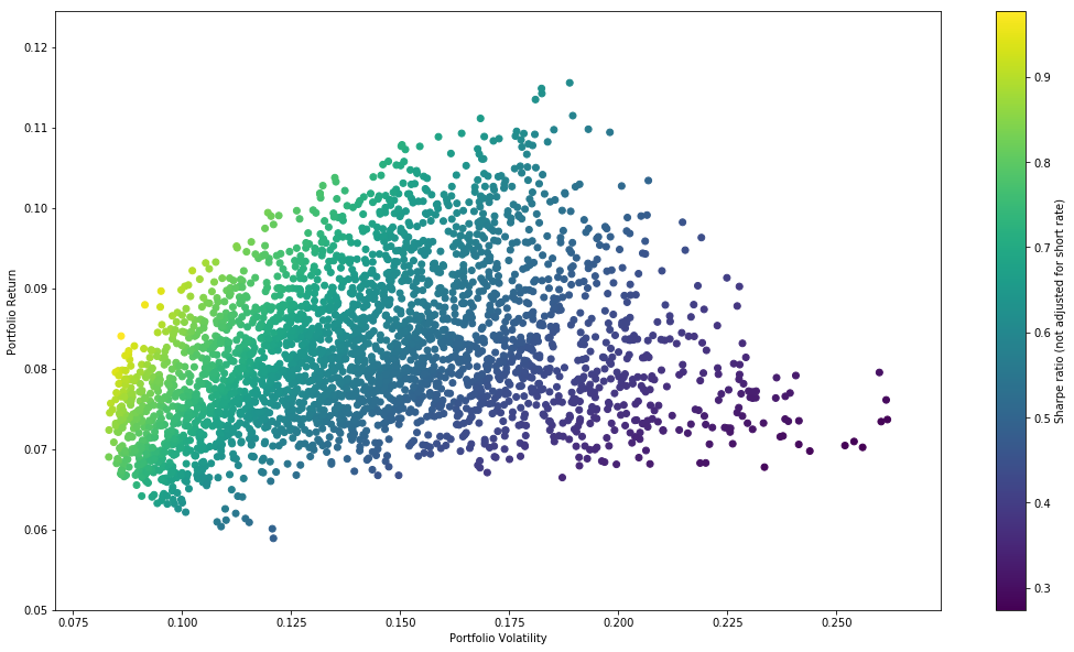
The resulting plot above is called the Markowitz Bullet. You might have noticed that the sprawl of dots - each representing one portfolio in the simulation - starts to form a sideways parabola. This shape lends itself extremely well to quadratic optimization functions because there is only one truly global minima and no other “false minima” that the optimization algorithm might get “stuck in”.
The Optimization Process
All optimization and minimization functions require some kind of metric to optimize on - usually this means minimizing something. This often involves tradeoffs because even though multi-variables can be considered, typically you can only minimize on score metric. In this example, we’re going to try optimizing on three seperate metrics just to get the hang of this. The metrics will be:
- Sharpe Ratio: Risk adjusted returns. This will create the portfolio with the highest return per unit of incurred risk.
- Variance (risk): Purely risk. This will create the portfolio with the lowest risk
- Pure Return: Purely return. This will create the portfolio with the highest return, regardless of risk.
To do this, let’s define functions that will generate all of these metrics for us and package them into a dictionary that we can pass to our soon-to-be created minimization functions.
def portfolio_stats(weights, returns):

    '''
    We can gather the portfolio performance metrics for a specific set of weights.
    This function will be important because we'll want to pass it to an optmization
    function to get the portfolio with the best desired characteristics.

    Note: Sharpe ratio here uses a risk-free short rate of 0.

    Paramaters:
    -----------
        weights: array,
            asset weights in the portfolio.
        returns: dataframe
            a dataframe of returns for each asset in the trial portfolio

    Returns:
    --------
        dict of portfolio statistics - mean return, volatility, sharp ratio.
    '''

    # Convert to array in case list was passed instead.
    weights = np.array(weights)
    port_return = np.sum(returns.mean() * weights) * 252
    port_vol = np.sqrt(np.dot(weights.T, np.dot(returns.cov() * 252, weights)))
    sharpe = port_return/port_vol

    return {'return': port_return, 'volatility': port_vol, 'sharpe': sharpe}
Next, if we want to optimize based on the sharpe ratio we need to define a function that returns only the sharpe ratio. Since our optimization functions naturally seek to minimize, we can minimize one of two quantities: The negative of the sharpe ratio, (or 1/(1+Sharpe Ratio). Accordingly, if the sharpe ratio increases both of these quantities will decrease. We’ll choose the negative of sharpe for this example.
Minimization Functions
def minimize_sharpe(weights, returns):
    return -portfolio_stats(weights)['sharpe']
def minimize_volatility(weights, returns):
# Note that we don't return the negative of volatility here because we
# want the absolute value of volatility to shrink, unlike sharpe.
return portfolio_stats(weights)['volatility'] def minimize_return(weights, returns):
return -portfolio_stats(weights)['return]The next thing we need to is introduce the optimization function we’ll use, and show how to seed the initial constraints, bounds, and parameters!
The Optimization Function
The scipy.optimize function accepts several parameters in order to optimize on your desired variable. Some of these are especially important in the portfolio optimization process.
- constraints: In this case, our key constraint is that all the portfolio weights should sum to 1.0. What this means, practically, is that all of our cash should be invested in an asset or ETF.
- bounds: Bounds is going to refer to how much of our portfolio one asset can take up, from 0.0 to 1.0. 0.0 being a 0% position, and 1.0 being a 100% position (That stock or ETF is our only holding). Note that we can change this if we want so that we don’t take on too much concentration risk. Concentration risk is the loss of diversification benefits you can encouter if one stock or ETF takes up too much of your portfolio. In reality, you might want to set these bounds to (0, 0.2), which means a single stock can only take up a maximum of 20% of the portfolio.
- initializer: Initializer just sets the initial weights of the optimization algorithm so that it has a starting point. Here we’ll just set them so that each stock takes up an equal percentage of the portfolio.
Click here to see the detailed documentation for this function.
constraints = ({'type' : 'eq', 'fun': lambda x: np.sum(x) -1})
bounds = tuple((0,1) for x in range(num_assets))
initializer = num_assets * [1./num_assets,]

print (initializer)
print (bounds)
[0.2, 0.2, 0.2, 0.2, 0.2]
((0, 1), (0, 1), (0, 1), (0, 1), (0, 1))
import scipy.optimize as optimize
optimal_sharpe=optimize.minimize(minimize_sharpe,
                                 initializer,
                                 method = 'SLSQP',
                                 bounds = bounds,
                                 constraints = constraints)
print(optimal_sharpe)
The output we get looks like this.
     fun: -0.9855053843923874
     jac: array([-2.30282545e-04, -4.28661704e-04,  1.79314971e-01,  4.32737172e-04,
        9.32403825e-01])
 message: 'Optimization terminated successfully.'
    nfev: 50
     nit: 7
    njev: 7
  status: 0
 success: True
       x: array([4.56881960e-01, 1.50685149e-01, 0.00000000e+00, 3.92432892e-01,
       9.63567740e-17])
Our import variable here is the last line, x. These represent the portfolio weights that produce the best sharpe ratio! But we’re missing our ticker names, so we can just do something like this to add some meaning:
optimal_sharpe_weights=optimal_sharpe['x'].round(4)
list(zip(assets,list(optimal_sharpe_weights)))
[('TLT', 0.4569), ('GLD', 0.1507), ('SPY', 0.0), ('QQQ', 0.3924), ('VWO', 0.0)]
Now, by calling our portfolio_stats function we can quantify the performance using these weights.
So what have we done here? We’ve run the optimization function by maximizing the Sharpe Ratio (minimizing the negative of the Sharpe Ratio). Accordingly, the portfolio weights that are spit out will provide us with a portfolio optimized for Sharpe.
This tells us that a portfolio of 45.69% TLT, 15.07% GLD, and 39.24% QQQ will give us the best risk adjusted returns.
We can pull out the individual performance parameters of this portfolio accordingly.
optimal_stats = portfolio_stats(optimal_sharpe_weights)
print(optimal_stats)

print('Optimal Portfolio Return: ', round(optimal_stats['return']*100,4))
print('Optimal Portfolio Volatility: ', round(optimal_stats['volatility']*100,4))
print('Optimal Portfolio Sharpe Ratio: ', round(optimal_stats['sharpe'],4))
[0.08650428 0.08777656 0.9855054 ]
Optimal Portfolio Return: 8.6504
Optimal Portfolio Volatility: 8.7777
Optimal Portfolio Sharpe Ratio: 0.9855
The Efficient Frontier
The efficient frontier is defined as all the portfolios that maximize the return for a given level of volatility. There can only be one of these for each level of volatility, and when plotted forms a curve around the cluster of portfolio values.
What we do is we iterate through a series of target returns, and for each target return we find the portfolio with the minimal level of volatility. To do this, we’ll need to minimize volatility instead of the negative of the sharpe ratio. This process is exactly the same as the process for sharpe ratio, except we substitute in our minimizing function for volatility instead.
optimal_variance=optimize.minimize(minimize_volatility,
                                   initializer,
                                   method = 'SLSQP',
                                   bounds = bounds,
                                   constraints = constraints)

print(optimal_variance)
optimal_variance_weights=optimal_variance['x'].round(4)
list(zip(assets,list(optimal_variance_weights)))
And we get a familiar output…
     fun: 0.006703774377738298
     jac: array([0.0133528 , 0.01338956, 0.01350171, 0.01346032, 0.02028012])
 message: 'Optimization terminated successfully.'
    nfev: 112
     nit: 16
    njev: 16
  status: 0
 success: True
       x: array([0.52228601, 0.13092821, 0.30560919, 0.0411766 , 0.        ])

[('TLT', 0.5223),
 ('GLD', 0.1309),
 ('SPY', 0.3056),
 ('QQQ', 0.0412),
 ('VWO', 0.0)]
In the code above we had the optimization algorithm optimize a portfolio such that it has the least amount of risk. The output shows the asset weighting required to minimize risk with this set of assets. Note that this is only for one portfolio. To plot an efficient frontier we need to loop through a bunch of target returns and repeat the exact same process above. We can then collect these results and plot them to see our frontier line.
# Make an array of 50 returns betweeb the minimum return and maximum return
# discovered earlier.
target_returns = np.linspace(port_returns.min(),port_returns.max(),50)

# Initialize optimization parameters
minimal_volatilities = []
bounds = tuple((0,1) for x in weights)
initializer = num_assets * [1./num_assets,]

for target_return in target_returns:

    constraints = ({'type':'eq','fun': lambda x: portfolio_stats(x)['return']-target_return},
                   {'type':'eq','fun': lambda x: np.sum(x)-1})

    optimal = optimize.minimize(minimize_volatility,
                              initializer,
                              method = 'SLSQP',
                              bounds = bounds,
                              constraints = constraints)

    minimal_volatilities.append(optimal['fun'])

minimal_volatilities = np.array(minimal_volatilities)
Now we can plot these results!
import matplotlib.pyplot as plt

# initialize figure size
plt.figure(figsize=(18,10))

plt.scatter(port_vols,
            port_returns,
            c = (port_returns / port_vols),
            marker = 'o')

plt.scatter(minimal_volatilities,
            target_returns,
            c = (target_returns / minimal_volatilities),
            marker = 'x')

plt.plot(portfolio_stats(optimal_sharpe_weights)['volatility'],
         Portfolio_Stats(optimal_sharpe_weights)['return'],
         'r*',
         markersize = 25.0)

plt.plot(portfolio_stats(optimal_variance_weights)['volatility'],
         portfolio_stats(optimal_variance_weights)['return'],
         'y*',
         markersize = 25.0)

plt.xlabel('Portfolio Volatility')
plt.ylabel('Portfolio Return')
plt.colorbar(label='Sharpe ratio (not adjusted for short rate)')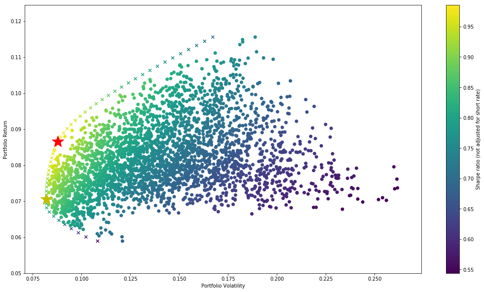
The Capital Market Line
In the above chart we can see the efficient frontier denoted by ‘x’s’. The big red star is the portfolio optimized for Sharpe Ratio, and the Yellow star is the portfolio is optimized to minimize variance (risk).
Now what we need to do is calculate the capital market line. We can accomplish this by calculating the line that intercepts the efficient frontier tangentially.
In order to do this, we need to make a better approximation of the efficient frontier and then calculate its first derivative along the approximated curve.
import scipy.interpolate as sci

min_index = np.argmin(minimal_volatilities)
ex_returns = target_returns[min_index:]
ex_volatilities = minimal_volatilities[min_index:]

var = sci.splrep(ex_returns, ex_volatilities)

def func(x):
    # Spline approximation of the efficient frontier
    spline_approx = sci.splev(x,var,der=0)
    return spline_approx

def d_func(x):
    # first derivative of the approximate efficient frontier function
    deriv = sci.splev(x,var,der=1)
    return deriv

def eqs(p, rfr = 0.01):

    #rfr = risk free rate

    eq1 = rfr - p[0]
    eq2 = rfr + p[1] * p[2] - func(p[2])
    eq3=p[1] - d_func(p[2])
    return eq1, eq2, eq3

# Initializing the weights can be tricky - I find taking the half-way point between your max return and max
# variance typically yields good results.

rfr = 0.01
m=  port_vols.max() / 2
l = port_returns.max() / 2

optimal = optimize.fsolve(eqs, [rfr,m,l])
print(optimal)
[0.01 0.89868124 0.08590308]
Note that solving for the capital market line equation can be finicky and you may have to play with it to get it right. Ultimately you’re looking for the capital market line to be tangential to the efficient frontier.
From experience, I find setting the first parameter equal to the risk free rate, the second paramter to half the max portfolio volatility, and the last parameter to half the max portfolio return seems to work.
Check to see the optimization function reduces all three equations to 0…
np.round(eqs(optimal),4)array([ 0., -0., 0.])
Now we’ll plot the capital market line, along with our spline approximation of the frontier along with all of the simulated portfolios.
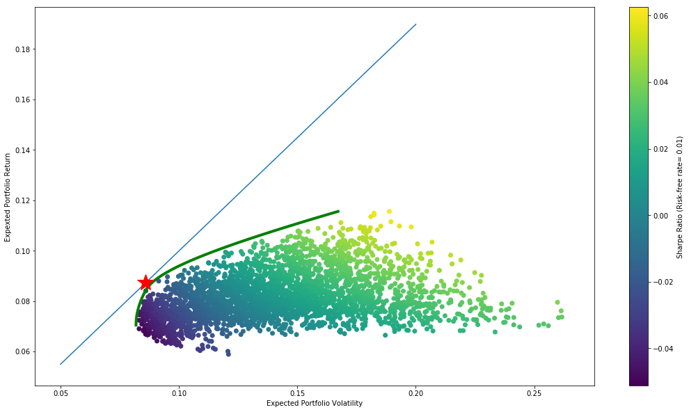
Now we can arrive at the weights of the markowitz optimal portfolio by running the optimization function again using the output from this function as our constraint.
constraints =(
    {'type':'eq','fun': lambda x: portfolio_stats(x)['return']-func(optimal[2])},
    {'type':'eq','fun': lambda x: np.sum(x)-1},
    )

result = optimize.minimize(minimize_volatility,
                           initializer,
                           method = 'SLSQP',
                           bounds = bounds,
                           constraints = constraints)

optimal_weights = result['x'].round(3)

portfolio = list(zip(assets, list(optimal_weights)))
print(portfolio)
[('TLT', 0.447), ('GLD', 0.15), ('SPY', 0.0), ('QQQ', 0.403), ('VWO', 0.0)]
By zipping together out asset list and our list of optimal weights we get a clear picture of how the optimal portfolio should be constructed.
In part two of this series we’ll tie everything together into a unified class function that allows us to analyze a portfolio of any number of assets we choose.
I hope you enjoyed this post!
Kevin Vecmanis