XGBoost Hyperparameter Tuning - A Visual Guide

May 11, 2019
Author :: Kevin Vecmanis

XGBoost is a very powerful machine learning algorithm that is typically a top performer in data science competitions. In this post I’m going to walk through the key hyperparameters that can be tuned for this amazing algorithm, vizualizing the process as we go so you can get an intuitive understanding of the effect the changes have on the decision boundaries.

In this article you will learn:

• What XGBoost is and what the main hyperparameters are
• How to plot the decision boundaries on simple data sets
• The effect of tuning n_estimators
• The effect of tuning max_depth
• The effect of tuning learning_rate
• The effect of tuning gamma
• The effect of tuning subsample size
• The effect of tuning min_child_weight
• How to conduct randomized search on XGBoost parameters

Table of Contents

• Introduction
• Function for plotting decision boundaries
• The n_estimators parameter
• The max_depth parameter
• The learning_rate parameter
• The gamma parameter
• The subsample parameter
• The min_child_weight parameter
• Conducting a randomized search on XGBoost hyperparameters

Introduction

If you’re like me, complex concepts are best grasped if you can see their effect visually. There are a lot of different machine learning algorithms and even more hyperparameters that need to be tuned. Although methods like randomized search and gridsearch negate some of the need to understand how the parameters work, it’s still a good idea to have an intuitive sense of their effect in case you’re not getting the performance you desire.

In this article, I’m going to focus on XGBoost. I’ve spent a lot of time with XGboost and its performance on most problems is exceptional. Most tuning guides and best practices you find on the internet provide numerial heuristics and rules-of-thumb for tuning the parameters. But what effect do these have on the decision boundaries? What does the effect look like? All else being equal, what effect does increasing the “gamma” parameter have on the decision boundary in different datasets? We’re going to explore this in detail in this post.

Attribution: The plotting solution used in this tutorial was borrowed from the great classifier comparison tutorial on the sklearn website here: classifier comparison.

In this article I adapt this to visualize the effect of hyperparameter tuning on key XGBoost parameters.

I’m going to change each parameter in isolation and plot the effect on the decision boundary. All hyperparameters will be set to their defaults, except for the parameter in question. We’ll do this for:

• n_estimators
• learning_rate
• min_samples_split
• max_depth
• gamma
• min_child_weight
• subsample

Plotting the decision boundaries

Note that it’s not important that you understand how this function works - I’m just including in the event you want to duplicate these results on your own.

import numpy as np
import matplotlib.pyplot as plt
from matplotlib.colors import ListedColormap
from sklearn.model_selection import train_test_split
from sklearn.preprocessing import StandardScaler
from sklearn.datasets import make_moons, make_circles, make_classification
from xgboost import XGBClassifier


def plot_decision_bounds(names,classifiers):
    
    '''
    This function takes in a list of classifier variants and names and plots the decision boundaries
    for each on three different datasets that different decision boundary solutions.
    
    Parameters: 
        names: list, list of names for labelling the subplots.
        classifiers: list, list of classifer variants for building decision boundaries.
        
    Returns: 
    
        None
    '''
    
    h = .02  # step size in the mesh
    X, y = make_classification(n_features=2, 
                               n_redundant=0, 
                               n_informative=2,
                               random_state=1, 
                               n_clusters_per_class=1)
    
    rng = np.random.RandomState(2)
    X += 2 * rng.uniform(size=X.shape)
    linearly_separable = (X, y)
    
    datasets = [make_moons(noise=0.3, random_state=0),
                make_circles(noise=0.25, factor=0.5, random_state=1),
                linearly_separable
                ]
    
    figure = plt.figure(figsize=(13, 8))
    i = 1
    # iterate over datasets
    for ds_cnt, ds in enumerate(datasets):
        # preprocess dataset, split into training and test part
        X, y = ds
        X = StandardScaler().fit_transform(X)
        X_train, X_test, y_train, y_test = \
            train_test_split(X, y, test_size=.4, random_state=42)
    
        x_min, x_max = X[:, 0].min() - .5, X[:, 0].max() + .5
        y_min, y_max = X[:, 1].min() - .5, X[:, 1].max() + .5
        xx, yy = np.meshgrid(np.arange(x_min, x_max, h),
                             np.arange(y_min, y_max, h))
    
        # just plot the dataset first
        cm = plt.cm.cool
        cm_bright = ListedColormap(['#FF0000', '#0000FF'])
        ax = plt.subplot(len(datasets), len(classifiers) + 1, i)
        if ds_cnt == 0:
            ax.set_title("Input data")
        # Plot the training points
        ax.scatter(X_train[:, 0], X_train[:, 1], c=y_train, cmap=cm_bright,
                   edgecolors='k')
        # and testing points
        ax.scatter(X_test[:, 0], X_test[:, 1], c=y_test, cmap=cm_bright, alpha=0.6,
                   edgecolors='k')
        ax.set_xlim(xx.min(), xx.max())
        ax.set_ylim(yy.min(), yy.max())
        ax.set_xticks(())
        ax.set_yticks(())
        i += 1
    
        # iterate over classifiers
        for name, clf in zip(names, classifiers):
            ax = plt.subplot(len(datasets), len(classifiers) + 1, i)
            clf.fit(X_train, y_train)
            score = clf.score(X_test, y_test)
    
            # Plot the decision boundary. For that, we will assign a color to each
            # point in the mesh [x_min, x_max]x[y_min, y_max].
            if hasattr(clf, "decision_function"):
                Z = clf.decision_function(np.c_[xx.ravel(), yy.ravel()])
            else:
                Z = clf.predict_proba(np.c_[xx.ravel(), yy.ravel()])[:, 1]
    
            # Put the result into a color plot
            Z = Z.reshape(xx.shape)
            ax.contourf(xx, yy, Z, cmap=cm, alpha=.8)
    
            # Plot also the training points
            ax.scatter(X_train[:, 0], X_train[:, 1], c=y_train, cmap=cm_bright,
                       edgecolors='k')
            # and testing points
            ax.scatter(X_test[:, 0], X_test[:, 1], c=y_test, cmap=cm_bright,
                       edgecolors='k', alpha=0.6)
    
            ax.set_xlim(xx.min(), xx.max())
            ax.set_ylim(yy.min(), yy.max())
            ax.set_xticks(())
            ax.set_yticks(())
            if ds_cnt == 0:
                ax.set_title(name)
            ax.text(xx.max() - .3, yy.min() + .3, ('%.2f' % score).lstrip('0'),
                    size=15, horizontalalignment='right')
            i += 1
    
    plt.tight_layout()
    plt.show()
    
    return

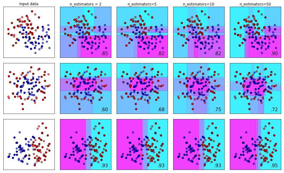
The n_estimators Parameter

With boosted tree models, models are trained sequentially - where each subsequence tree tries to correct for the errors made by the previous sequence of trees.

The `n_estimators_ parameter specifies how many sequential trees we want to make that attempt to correct for prior trees. The number of estimators required will depend on the size and complexity of your dataset, but you should be aware that the law of diminishing returns applies here. This means that most of your gains are going to happen early, and improvements with additional estimators will diminish over time.

names = ['n_estimators = 2', 'n_estimators = 5', 'n_estimators = 10', 'n_estimators = 50']
classifiers = [XGBClassifier(n_estimators = 2),
               XGBClassifier(n_estimators = 5),
               XGBClassifier(n_estimators = 10),
               XGBClassifier(n_estimators = 50)
               ]

plot_decision_bounds(names,classifiers)

The effect of tuning n_estimators from 2 to 50 can be seen below on three different types of toy datasets.

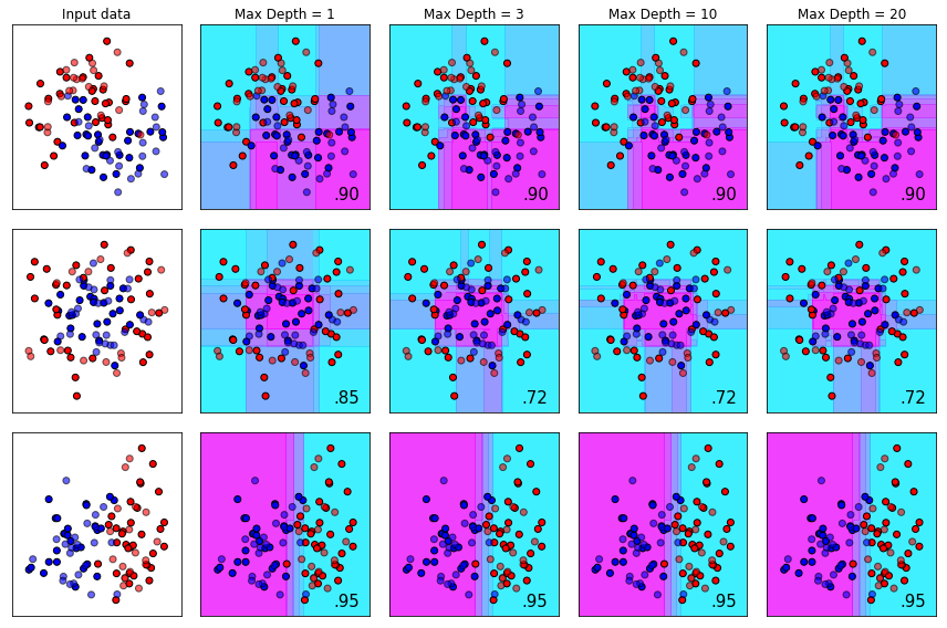
The max_depth Parameter

The max_depth parameter determines how deep each estimator is permitted to build a tree. Typically, increasing tree depth can lead to overfitting if other mitigating steps aren’t taken to prevent it. Like all algorithms, these parameters need to be view holistically. For datasets with complex structure, a deep tree might be required - other parameters like min_child_weight can be increased to mitigate chances of overfitting.

names = ['Max Depth = 1', 'Max Depth = 3', 'Max Depth = 10', 'Max Depth = 20']
classifiers = [XGBClassifier(max_depth=1),
               XGBClassifier(max_depth=3),
               XGBClassifier(max_depth=10),
               XGBClassifier(max_depth=20)
               ]

plot_decision_bounds(names,classifiers)

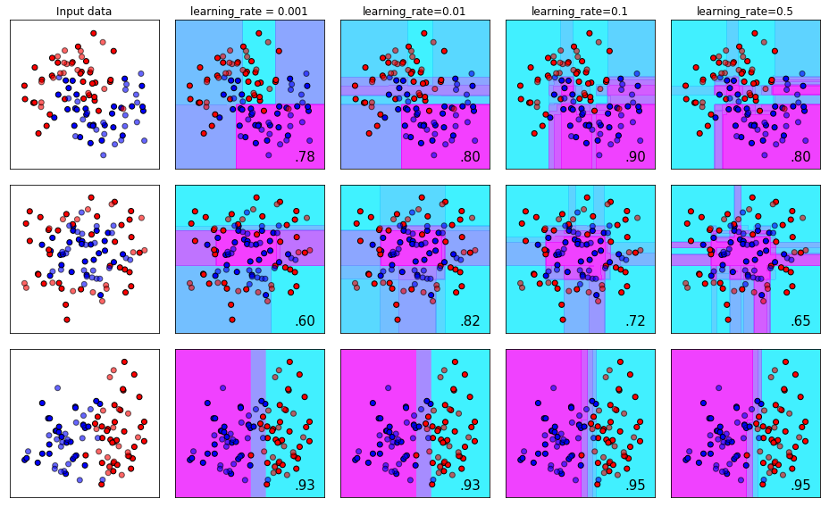
The learning_rate Parameter (AKA eta)

The learning_rate parameter (also referenced in XGboost documentation as eta) controls the magnitude of change that is permitted from one tree to the next. To conceptualize this, you can think of this like learning the golf swing. If you slice the ball after your first shot at your golf lesson, it doesn’t mean you need to dramatically change the way you’re hitting the ball. Typically you want to make small, purposeful adjustments after each shot until you finally get the desired flight bath.

The flip side of this is that you definitely _do want to make adjustments after each shot if you’re not hitting it correctly. How much adjustment between shots depends on the person, the coach, and how bad your shot is! If you change too much after each attempt you may run the risk of discaring the aspects of your swing that were actually good. Dramatic alterations between each shot, you can imagine, might result in a completely ineffective learning process.

names = ['learning_rate = 0.001', 'learning_rate = 0.01', 'learning_rate = 0.1', 'learning_rate = 0.5']
classifiers = [XGBClassifier(learning_rate = 0.001),
               XGBClassifier(learning_rate = 0.010),
               XGBClassifier(learning_rate = 0.100),
               XGBClassifier(learning_rate = 0.500)
               ]

plot_decision_bounds(names,classifiers)

The gamma Parameter

The gamma is an unbounded parameter from 0 to infinity that is used to control the model’s tendency to overfit. This parameter is also called min_split_loss in the reference documents. Thing of gamma as a complexity controller that prevents other loosely non-conservative parameters from fitting the trees to noise (overfitting).

Finding a good gamma, like most of the other parameters, is very dependent on your dataset and how the other parameters are configured. Gamma is often very useful when you have an extremely deep tree and overfitting would be inevitable without mitigating factors.

To use another analogy - imagine you have a huge tree in your front that is growing out of control. Leaves everywhere, overtaking power lines, and encroaching on your house! You can think of gamma as the arborist that comes to your house to prune the branches and leaves to get the tree back under control.

names = ['gamma = 0', 'gamma = 0.5', 'gamma = 2', 'gamma = 10']
classifiers = [XGBClassifier(gamma=0),
               XGBClassifier(gamma=0.5),
               XGBClassifier(gamma=2),
               XGBClassifier(gamma=10)
               ]

plot_decision_bounds(names, classifiers)

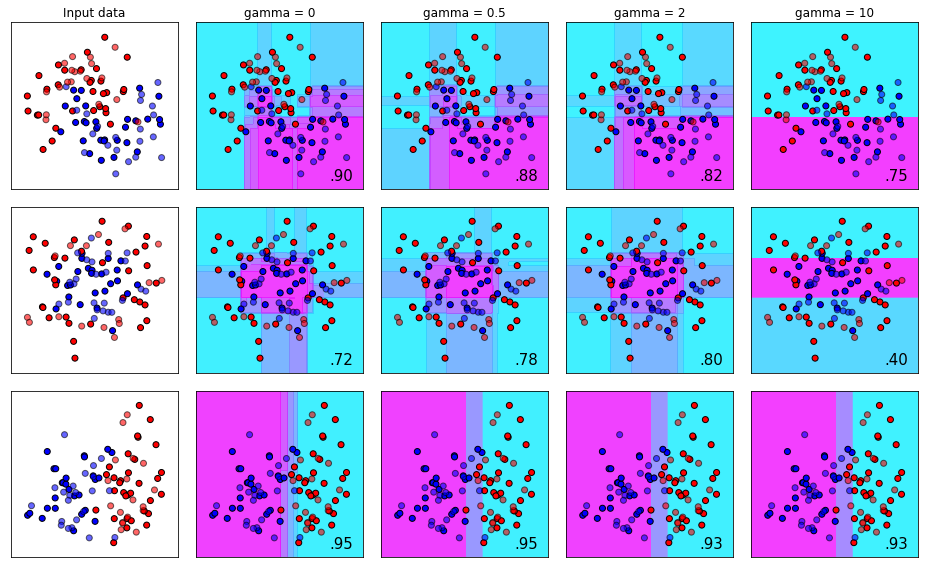
In this sequences, look at the first and second rows. As we increase gamma, the subtleties in the decision making parameters start to disappear and they become more blunt as we go further right. Also note that in the middle row, increasing gamma from 0 to 2 improved our accuracy from 0.72 to 0.80, but an additional increase in gamma cratered our score down to 0.40. The takeaway here is that if Gamma is needed, in most cases it will only help up to a certain point and then become a hindrance to your model’s ability to generalize.

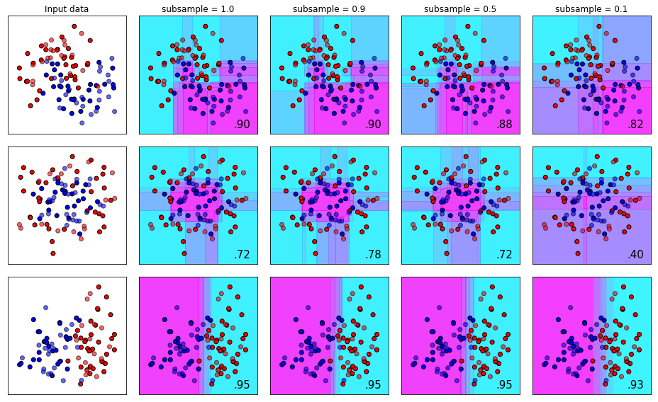
The subsample Parameter

The subsample parameter determines how much of the initial dataset is fair game for random sampling during each iteration of the boosting process. The default here is set to 1.0, which means each iteration of the training process can sample 100% of the data.

This is another useful parameter for controlling overfit (noticing a theme yet?). Why does this control overfit? Well, recall from the section on n_estimators that each stage of the boosting process attempts to correct the errors of the prior sequence of trees. If each tree in the sequence is training on a slightly difference dataset than the trees prior, the error correction process starts to generalize across “new” samples during the training phase.

Using our golf analogy again - imagine practicing on a real golf course instead of a driving range where every should is roughly the same. Each shot on a real golf course is a slightly different version of the same bio-mechanical movement. In theory, this would give you a golf swing that “generalizes” well to different situations other than the comparatively pristine conditions of a driving range tee block.

names = ['subsample = 1.0', 'subsample = 0.9', 'subsample = 0.5', 'subsample = 0.1']
classifiers = [XGBClassifier(subsample = 1.0),
               XGBClassifier(subsample = 0.9),
               XGBClassifier(subsample = 0.5),
               XGBClassifier(subsample = 0.1)
               ]

plot_decision_bounds(names,classifiers)

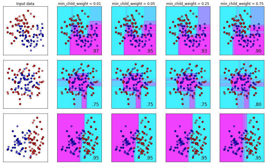
The min_child_weight Parameter

The number of samples required to form a leaf node (the end of a branch). A leaf node is the termination of a branch and therefore the decision node of what class a sample belongs to.

Imagine you have a dataset for classifying cats and dogs. Suppose further that the dataset has 1000 samples, and there is a perfect split between dogs and cats - meaning there are 500 cases of each.

If you set the min_child_weight parameter to be 500, you would be forcing the algorithm to find one decision path that is common to the entirety of each class. Depending on your features this might be entirely possible - but chances are it’s not. The flip side of this is setting min_child_weight to 1. Meaning each decision branch only needs one sample in order for the branch to be valid. This would result in extreme overfit, because the algorithm (with enough features) would be unconstrained from building a unique path to describe each sample.

Remember, the goal of making machine learning models is to build something that generalizes well to new data. You don’t want to force to find a common branch for all of the samples, nor do you want to give it the leeway to fit itself to noise.

With XGBoost, you can specify this parameter as a float as well. If you do, it will use a percentage of samples to determine leaf nods. For example, specificying 0.9 would mean “90% of the samples need to be in a leaf in order for the leaf to be valid”.

names = ['min_child_weight = 0.01', 'min_child_weight = 0.05', 'min_child_weight = 0.25', 'min_child_weight = 0.75']
classifiers = [XGBClassifier(min_child_weight = 0.01),
               XGBClassifier(min_child_weight = 0.05),
               XGBClassifier(min_child_weight = 0.25),
               XGBClassifier(min_child_weight = 0.75)
               ]

plot_decision_bounds(names,classifiers)

Randomized hyperparameter search with XGBoost

The following is a code recipe for conducting a randomized search across XGBoost’s entire parameter search space. It will randomly sample the parameter space 500 times (adjustable) and report on the best space that it found when it’s finished. The recipe uses 10-fold cross validation to generate a score for each parameter space. Note that I haven’t included data in this recipe.

import time
import numpy as np
from xgboost import XGBClassifier
from sklearn.model_selection import RandomizedSearchCV
from sklearn.model_selection import KFold
from sklearn.metrics import accuracy

start_time=time.time()

#### Create X and Y training data here.....


# grid search
model = XGBRegressor()

param_grid = {
        'max_depth': [3, 4, 5, 6, 7, 8, 9, 10, 11, 12]
        'min_child_weight': np.arange(0.0001, 0.5, 0.001),
        'gamma': np.arange(0.0,40.0,0.005),
        'learning_rate': np.arange(0.0005,0.3,0.0005),
        'subsample': np.arange(0.01,1.0,0.01),
        'colsample_bylevel': np.round(np.arange(0.1,1.0,0.01),
        'colsample_bytree': np.arange(0.1,1.0,0.01),
{

kfold = KFold(n_splits=10, shuffle=True, random_state=10)
grid_search = RandomizedSearchCV(model, param_grid, scoring="accuracy", n_iter = 500, cv=kfold)
grid_result = grid_search.fit(X,Y)

# summarize results
print("Best: %f using %s" % (grid_result.best_score_, grid_result.best_params_))
means = grid_result.cv_results_[ 'mean_test_score' ]
stds = grid_result.cv_results_[ 'std_test_score' ]
params = grid_result.cv_results_[ 'params' ]

print(time.time()-start_time)

Summary

We have visually demonstrated the effect of tuning some of the key parameters for XGBoost. It’s important to keep in mind that the optimal values for these will depend entirely on the dataset.

I left with you a sample that can be used to conduct a random search through most of the key parameters for XGBoost’s parameter space.

For more information on XGBoost, visist the official site here: XGBoost Website

Thanks for reading!

Kevin Vecmanis