Clustering Frequency Domain Data

Jul 18, 2019
Author :: Kevin Vecmanis

Unsupervised clustering algorithms can be a great way to explore any structure that is inherent to the data and perhaps not immediately obvious to the analyst.

Introduction
Problem Statement
Data Exploration
Applying Fourier Transform to Obtain Frequency Spectrum of Each Signal
Apply KMeans Clustering Algorithm
Color coding the spectra according to their cluster

Introduction

The following exercise was actually from a take-home coding assignment from a company (who remains unnamed) I was interviewing with.

Problem Statement

A zip file was provided with 40 files - all of them .npy object files (Numpy objects). The following instructions were provided:

Use a clustering method, to cluster the attached data into 3 groups.

Dataset:

each data sample is a 1D signal containing 2400 points

Expected Results:

What is the method used for the clustering? How is it decided which method to use?
Visualization of the clusters with the labels of the data point
The developed codes

Hint: You may need to focus on a part of the signal for the best clustering

The file names were as follows:

 '2018-10-15_11-31-41-PASSTHROUGH-12-59-31.npy',
 '2018-10-18_14-25-40-PASSTHROUGH-12-59-31.npy',
 '2018-10-15_11-30-03-PASSTHROUGH-12-59-31.npy',
 '2018-10-15_11-40-25-PASSTHROUGH-12-59-31.npy',
 '2018-10-18_14-20-19-PASSTHROUGH-12-59-31.npy',
 '2018-10-15_11-55-18-PASSTHROUGH-12-59-31.npy',
 '2018-10-18_14-10-19-PASSTHROUGH-12-59-31.npy',
 '2018-10-15_11-36-36-PASSTHROUGH-12-59-31.npy',
 '2018-10-15_11-53-51-PASSTHROUGH-12-59-31.npy',
 '2018-10-18_14-56-57-PASSTHROUGH-12-59-31.npy',
 '2018-10-18_14-06-45-PASSTHROUGH-12-59-31.npy',
 '2018-10-18_14-29-51-PASSTHROUGH-12-59-31.npy',
 '2018-10-15_12-02-56-PASSTHROUGH-12-59-31.npy',
 '2018-10-15_11-38-01-PASSTHROUGH-12-59-31.npy',
 '2018-10-18_14-07-48-PASSTHROUGH-12-59-31.npy',
 '2018-10-18_14-30-51-PASSTHROUGH-12-59-31.npy',
 '2018-10-18_14-00-47-PASSTHROUGH-12-59-31.npy',
 '2018-10-15_11-44-00-PASSTHROUGH-12-59-31.npy',
 '2018-10-18_13-58-38-PASSTHROUGH-12-59-31.npy',
 '2018-10-18_14-19-14-PASSTHROUGH-12-59-31.npy',
 '2018-10-15_11-48-43-PASSTHROUGH-12-59-31.npy',
 '2018-10-15_11-39-18-PASSTHROUGH-12-59-31.npy',
 '2018-10-15_11-45-03-PASSTHROUGH-12-59-31.npy',
 '2018-10-18_14-32-01-PASSTHROUGH-12-59-31.npy',
 '2018-10-18_14-26-39-PASSTHROUGH-12-59-31.npy',
 '2018-10-15_11-56-44-PASSTHROUGH-12-59-31.npy',
 '2018-10-18_14-54-45-PASSTHROUGH-12-59-31.npy',
 '2018-10-15_12-05-27-PASSTHROUGH-12-59-31.npy',
 '2018-10-18_14-35-02-PASSTHROUGH-12-59-31.npy',
 '2018-10-18_14-18-15-PASSTHROUGH-12-59-31.npy',
 '2018-10-18_14-55-53-PASSTHROUGH-12-59-31.npy',
 '2018-10-18_14-38-29-PASSTHROUGH-12-59-31.npy',
 '2018-10-18_14-13-11-PASSTHROUGH-12-59-31.npy',
 '2018-10-18_14-05-15-PASSTHROUGH-12-59-31.npy',
 '2018-10-18_14-24-33-PASSTHROUGH-12-59-31.npy',
 '2018-10-18_14-02-47-PASSTHROUGH-12-59-31.npy',
 '2018-10-18_14-11-51-PASSTHROUGH-12-59-31.npy',
 '2018-10-15_12-04-10-PASSTHROUGH-12-59-31.npy',
 '2018-10-15_11-33-03-PASSTHROUGH-12-59-31.npy',
 '2018-10-18_14-36-01-PASSTHROUGH-12-59-31.npy'

High-Level Solution Methodology

My approach to solving this problem was as follows:

Window the time series signal to the active components.
Get frequency domain representation for each of the 40 windowed signals.

Data Exploration

The first thing I decided to do was to visualize the data provided in each .npy file. Visually, the signals appear to be roughly the same type - my suspicion is that they’re intended to mimic some sort of radio or radar reflection signal. To visualize the raw signals I did the following:

import numpy as np
import pandas as pd
import matplotlib.pyplot as plt
import scipy as sp
import scipy.fftpack
from os import listdir

#Set figure size for matplotlib
plt.rcParams['figure.figsize'] = [20, 12]

for file in files:
    x = np.load(file)
    plt.plot(x)
plt.title('Raw data plotted on same scale')
plt.show()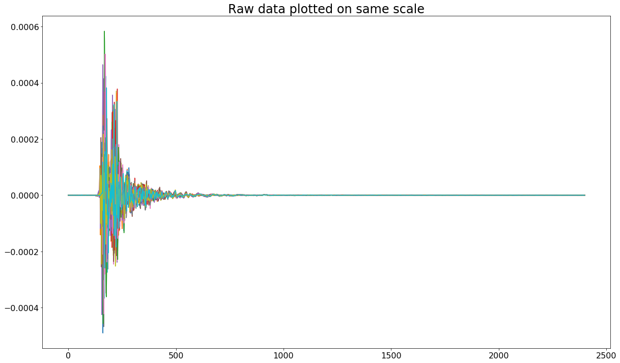

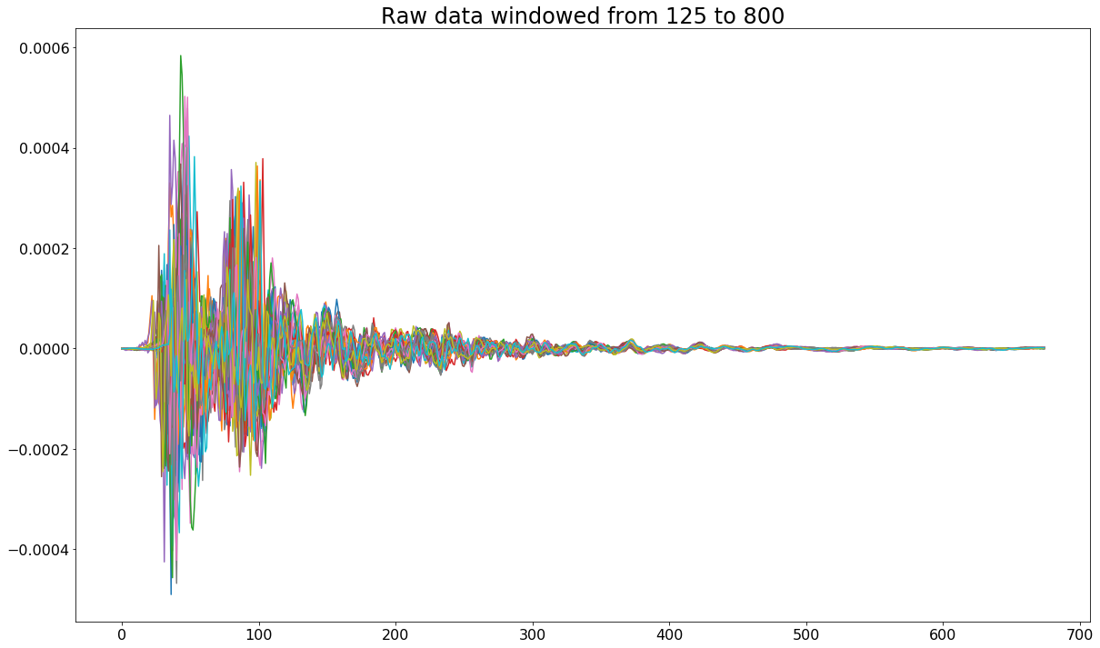
raw_data

Because the body of the signals begins and ends in roughly the same location, I decided to trim them from index 125 to index 800 to arrive at the following.

windowed_raw_data

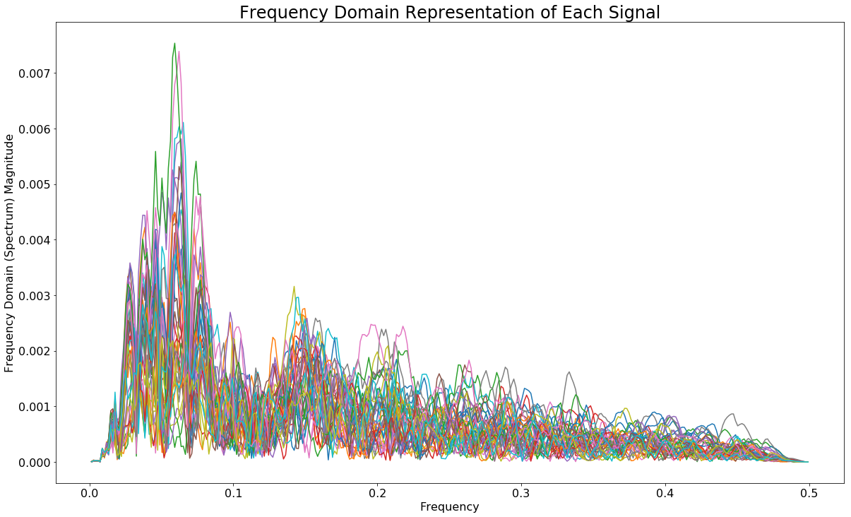
Applying Fourier Transform to Obtain Frequency Spectrum of Each Signal

The next step in the process was to convert each signal to the frequency domain which can then be used in the KMeans clustering algorithm. This was achieved as follows:

freqs = sp.fftpack.fftfreq(675) # 675 is the length of the new window. (800-125)
spectra = []
fig, ax = plt.subplots()

# Because frequency domain is symmetrical, take only positive frequencies
i = freqs > 0
for signal in data:
    X = sp.fftpack.fft(signal)  
    ax.plot(freqs[i], np.abs(X)[i])
    spectra.append(np.abs(X)[i])

ax.set_xlabel('Frequency')
ax.set_ylabel('Frequency Domain (Spectrum) Magnitude')
ax.set_title('Frequency Domain Representation of Each Signal')

frequency_domain

Apply KMeans Clustering Algorithm

The next step in the process was to apply a clustering algorithm to the 40 sets of frequency spectra.

from sklearn.cluster import KMeans
kmeans = KMeans(3, max_iter = 1000, n_init = 100)
kmeans.fit_transform(spectra)
predictions = kmeans.predict(spectra)
predictions

Output:

array([1, 1, 2, 1, 0, 1, 2, 1, 2, 0, 0, 2, 2, 1, 0, 1, 0, 2, 2, 0, 0, 2,
       1, 2, 0, 1, 2, 0, 2, 2, 0, 1, 0, 2, 2, 0, 0, 1, 2, 1], dtype=int32)

Color coding the spectra according to their cluster

fig2, ax2 = plt.subplots()
for spectra_id, color in enumerate(['red','blue','green']):
    mask = list(np.where(predictions==spectra_id)[0])
    print(mask)
    for elem in mask:
        ax2.plot(freqs[i], spectra[elem], color=color)

ax2.set_xlabel('Frequency')
ax2.set_ylabel('Frequency Domain (Spectrum) Magnitude')

frequency_clustered

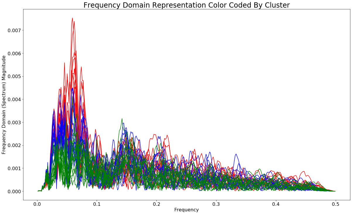
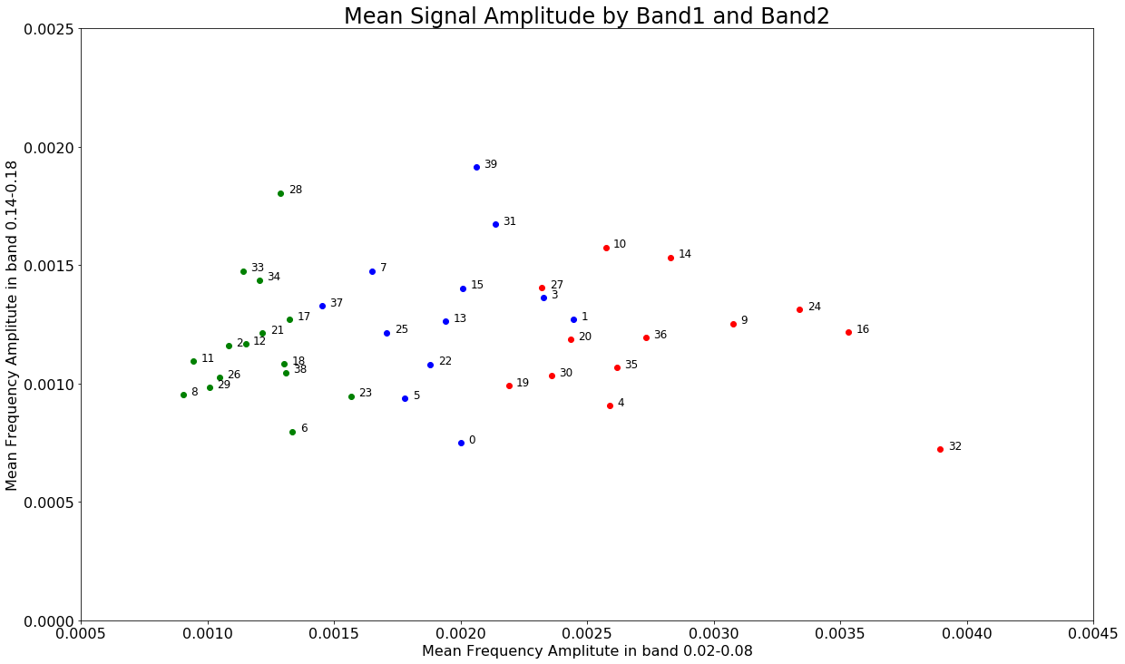
The next thing I want to do is plot each of these spectra on a two dimensional plot where each dimension is one of the two dominant frequency bands - roughly 0.0050 - 0.006 (band1) and 0.14-0.16 (band2).

positive_frequencies = freqs[i]
band1 = np.where(np.logical_and(positive_frequencies>=0.02, positive_frequencies<=0.08))
band2 = np.where(np.logical_and(positive_frequencies>=0.14, positive_frequencies<=0.18))

x = []
y = [] 
for spectrum in spectra:
    x.append(np.mean(spectrum[band1]))
    y.append(np.mean(spectrum[band2])) 

fig3, ax3 = plt.subplots()
for spectra_id, color in enumerate(['red','blue','green']):
    mask = list(np.where(predictions==spectra_id)[0])
    for elem in mask:
        ax3.scatter(x[elem], y[elem], color=color)
        ax3.text(x[elem]+0.00003, y[elem], elem, fontsize=12)

ax3.set_ylim(0.000, 0.0025)
ax3.set_xlim(0.0005, 0.0045)
ax3.set_xlabel('Mean Frequency Amplitute in band 0.02-0.08')
ax3.set_ylabel('Mean Frequency Amplitute in band 0.14-0.18')
ax3.set_title('Mean Signal Amplitude by Band1 and Band2')