Binary Tree Methods in Python
Author :: Kevin Vecmanis
In this post I show you a class for creating binary trees (and a cool way to display them!), as well as some methods for analyzing binary trees. Enjoy!
In this article you will learn about:
- What binary trees are and what they are good for
- How to build them from scratch in Python
- How to insert into a binary tree
- How to find the depth of a tree
- How to traverse the tree in different ways
- How to find the maximum value in a tree
- What a balanced tree is, and how to balance one that is unbalanced
- What binary heaps are and how to use them in Python
Table of Contents
- Introduction
- Creating and Inserting into a Binary Tree
- Balancing a Binary Tree
- In-Order Traversal
- Post-Order and Pre-Order Traversals
- Find the Size of a Binary Tree
- Find the Maximum Depth of the Tree
- Find the Number of Leaf Nodes in the Tree
- Binary Heaps
Introduction: What are Binary Trees?

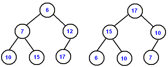
A binary tree is a data structure where each node has at most two children, as shown in the diagram above. Binary Trees are incredibly useful in certain applications because they’re intuitive and can perform fast search operations. Because the structure is repeating, the code necessary to execute tasks on binary trees is often compact and recursive.
Creating and Inserting into Binary Tree
To follow along with this code, you can clone the binary_tree Node class from this Github repo: Binary Trees
A binary tree can be created fairly easily by declaring the following class:
class Node:
    """A class for creating a binary tree node and inserting elements.

       Attributes:
       -----------
       data : int, str
            The value that exists at this node of the tree.  eg. tree=Node(4) initializes a tree with
            a stump integer value of 4.

       Methods:
       --------
       insert(self, data) : Inserts a new element into the tree.
    """

    def __init__(self, data):
        self.data = data
        self.right = None
        self.left = None


    def insert(self, data):
        if self.data == data:
            return
        elif self.data < data:
            if self.right is None:
                self.right = Node(data)
            else:
                self.right.insert(data)
        else: # self.data > data
            if self.left is None:
                self.left = Node(data)
            else:
                self.left.insert(data)
Note: There is a helper method called display() that I’ve left out here, but it can be found in the github repo!
This lets us create a binary tree and insert values into it like this:
>>> from binary_trees_class import Node
>>> tree = Node(10)
>>> tree.display()
10
When inserting values into a binary tree, duplicates are not allowed by design. If the value you’re inserting is smaller than the root node, it goes to the left. If it’s larger, it goes to the right.
>>> tree.insert(5)
>>> tree.insert(20)
>>> tree.display()
  10_
 /   \
5     20
To grow out a bigger tree, we can loop through a list to perform these insertions:
>>> values = [1,5,20,99,45,12,44,41,18,7,11,19,82,87]
>>> for value in values:
...     tree.insert(value)
...
>>> tree.display()
   _10_________
  /            \
  5       ____20___________
 / \     /                 \
1   7    12_           ____99
       /   \         /
      11  18_       45_
             \     /   \
             19    44  82_
                  /       \
                 41       87
Like trees in real life, if they’re left to grow by their own devices they can become unruly. One of the main applications of binary trees is binary search. Binary search allows you to find a value in at most log2n operations. What does this mean?
Well, imagine we have an array of numbers that has 32 values in it. To find a value in this array, the worst case scenario is that we traverse the array, one at a time, and the value we’re looking for is at the end of the array. This will take us 32 operations to find.
With a properly structured binary tree, this will take us at most 5 operations (log2(32) = 5). This is also the depth of the tree. In a binary tree, our worst case scenario is that the value we’re searching for resides in one of the leaf nodes of the tree - in other words, it’s at the bottom and has no children. In our tree right now, 41, 87, 19, 11, 7, and 1 are all leaf nodes.
Notice that before I mentioned the caveat properly structured tree to achieve this performance. Think about our list - our maximum depth is 5 right now, but we don’t have 32 values - we only have 15 values. The way our tree is structured right now, it would take 5 operations to find the values 41 and 87. But log2(15) ~ 3.9. We’re losing some performance here because our tree isn’t balanced. We can balance our tree by putting the median value (in size) at the top (root) node of the tree.
Let’s introduce a new method to do this - but first let’s define a method that can check if our tree is balanced. What is a balanced Tree?
Balancing a Binary Tree
A binary tree is balanced if:
- It’s empty.
- If it’s not empty:
- The left sub tree is balanced, and
- The right subtree is balanced, and
- The difference in depth between left and right is <=1
def is_balanced(root):
    '''
    Method for determining if a binary tree is balanced.

    A binary tree is balanced if:
        - it's empty
        - the left sub tree is balanced
        - the right subtree is balanced
        - the difference in depth between left and right is <=1

    Parameters:
    ____________
    root : the node object, below which the definition of 'balanced' will be applied.
    '''
    if root is None:
        return True
    return is_balanced(root.right) and is_balanced(root.left) and abs(get_height(root.left) - get_height(root.right)) <= 1
Now we can confirm if our tree is balanced:
>>> is_balanced(tree)
False
To balance the tree, we’re going to store all the values in an array and then execute the following algorithm:
- Find the middle value of the array
- Set that as the root node
- Build a tree with the remainder of the array using our regular insertion algorithm.
To build the array, we’re going to do an in-order traversal of the tree. This is done by:
- Traversing the left subtree
- Visit the root
- Traverse the right subtree
In-Order Traversal
def inorder_traversal(root):
    '''
    Return an array of tree elements using inorder traversal.
    In-order traversal = Left-->Root-->Right
    '''
    res = []
    if root:
        res = inorder_traversal(root.left)
        res.append(root.data)
        res = res + inorder_traversal(root.right)
    return res
Our resulting array looks like this:
inorder_traversal(tree)
[1, 5, 7, 10, 11, 12, 18, 19, 20, 41, 44, 45, 82, 87, 99]
Notice that our array is already sorted! This is the value of the inorder traversal, and its primary use case. An inorder traversal, just like the name implies, returns the values of the tree in order. Nice right?
Balance a Binary Tree
def balance_tree(array):
    '''
    Balances an unbalanced binary tree in O(n) time from the inorder traversal
    stored in an array
    steps:
        - Take inorder traversal of existing tree and store in array.
        - Find value at mid point of this array.
        - create new binary tree using this midpoint as root node.
    '''
    if not array:
        return None

    midpoint = len(array) // 2
    new_root = Node(array[midpoint])
    new_root.left = balance_tree(array[ : midpoint])
    new_root.right = balance_tree(array[midpoint + 1 :])
    return new_root
Now what we can do is pass our inorder traversal to the balance_tree() method and we’ll get our balanced tree spit out the other side.
>>> balanced_tree = balance_tree(inorder_traversal(tree))
>>> balanced_tree.display()

     ______19_______
    /               \
  _10___         __45___
 /      \       /       \
 5     12_     41_     87_
/ \   /   \   /   \   /   \
1 7  11  18  20  44  82  99
Perfect! Now we have a balanced tree that can execute value searches in true log2n time. This is how most relational database systems produce an index, often called a btree index. Binary Tree indexes are what allows relational database programs to execute such fast search queries - but only if the index exists! Database reindexing is the process of rebuilding this binary tree when new entries are made to the database table. With this in mind, you can start to understand some of the trade-offs required with database binary tree indexes. Since it takes O(n) time to rebalance a tree, our time complexity can quickly explode if we’re reindexing a database that has values added to it at a high frequency.
Post-Order and Pre-Order Traversals
Where an in-order traversal returns an array that is sorted in order, there are two other types of traversals as well - pre-order and post-order.
Pre-Order Traversal
A pre-order traversal traverses the tree in this order: Root–>Left–>Right. You use this type of traversal if you’re looking to take an exact copy of a tree’s structure. Let’s see an example…
def preorder_traversal(root):
    '''
    Returns an array of tree elements using pre order traversal.
    Pre order is often used to copy a tree
    Pre-order traversal = Root-->Left-->Right
    '''
    res=[]
    if root:
        res.append(root.data)
        res = res + preorder_traversal(root.left)
        res = res + preorder_traversal(root.right)

    return res
>>> preorder_traversal(tree)
[10, 5, 1, 7, 20, 12, 11, 18, 19, 99, 45, 44, 41, 82, 87]
>>> tree.display()
_10_________
/ \
5 ____20___________
/ \ / \
1 7 12_ ____99
/ \ /
11 18_ 45_
\ / \
19 44 82_
/ \
41 87
Post-Order Traversal
A post-order traversal traverses the tree in this order: Left–>Right–>Root. This would be used when you want to begin deleting elements from the tree.
def postorder_traversal(root):
    '''
    Returns an array of tree elements using post order traversal.
    Post order is often used to delete tree elements.
    Post-order traversal = Left-->Right-->Root
    '''
    res=[]
    if root:
        res=postorder_traversal(root.left)
        res = res + postorder_traversal(root.right)
        res.append(root.data)

    return res
>>> postorder_traversal(tree)
[1, 7, 5, 11, 19, 18, 12, 41, 44, 87, 82, 45, 99, 20, 10]
>>> tree.display()
_10_________
/ \
5 ____20___________
/ \ / \
1 7 12_ ____99
/ \ /
11 18_ 45_
\ / \
19 44 82_
/ \
41 87
Find the Size of a Binary Tree
To get the size of the tree (number of nodes in it), we find the size of the left tree and the size of the right tree and add them. Then we add 1 because we don’t want to forget about the parent node.
def size(root):
    '''
    Compute the total number of nodes in a tree.
    '''
    if root is None:
        return 0
    else:
        return (size(root.left) + 1 + size(root.right))
>>> size(tree)
15
Find the Maximum Depth of the Tree
This is another recursive operation…
def get_height(root):
    '''
    Returns the maxium depth of the tree.

    Parameters:
    ___________
    root : the node object, below which maximum depth will be calculated.
    '''
    if root is None:
        return 0
    return 1 + max(get_height(root.left), get_height(root.right))
>>> get_height(tree)
6
>>> get_height(balanced_tree)
4
Find the Number of Leaf Nodes in the Tree
The function will return the number leaf nodes in the tree (nodes without children)
def get_leaf_count(node):
    '''
    Count the number of leaf nodes in a tree.

    Parameters:
    ___________
    node : object
        a binary tree object
    '''
    if node is None:
        return 0
    if(node.left is None and node.right is None):
        return 1
    else:
        return get_leaf_count(node.left) + get_leaf_count(node.right)
>>> get_leaf_count(tree)
6
>>> get_leaf_count(balanced_tree)
8
Binary Heaps
A binary heap is a special type of binary tree that satisfies one of two special ordering patterns:
- Max Heap: The value of each node is less than or equal to the value of its parent, with the maximum-value element at the root.
- Min Heap: The value of each node is greater than or equal to the value of its parent, with the minimum-value element at the root.
Heaps are what’s called “partially ordered” structures. Although either the minimum or maximum value can reliably found at the root node, the rest of the tree isn’t guaranteed to be in order.
Heaps are especially useful for implementing priority queues, or any situations where quick access is needed to the maximum or minimum value in a collection.
In python, you can implement a heap using the built in library heapq. As of this writing, the standard Python implementation of heap is a MinHeap. To get a MaxHeap, you can multiple all the values in the list by -1 and it will perform as a MaxHeap.
Creating the heap
heapify()
import heapq
>>> h = [14,6,12,56,1,14,29,44,88]
>>> heapq.heapify(h)
>>> print(h)
[1, 6, 12, 44, 14, 14, 29, 56, 88]
Note that althought the smallest element will always be at index 0, the rest of the list isn’t necessarily sorted. That being said, the heapq.heappop() method will always pop the smallest element (removed the element from the list)
Removing from the heap
heappop()
>>> heapq.heappop(h)
1
>>> heapq.heappop(h)
6
>>> heapq.heappop(h)
12
>>> heapq.heappop(h)
14
>>> heapq.heappop(h)
14
>>> heapq.heappop(h)
29
>>> h
[44, 56, 88]
Adding to the heap
heappush()
>>> heapq.heappush(h,16)
>>> h
[16, 44, 88, 56]
Summary
That’s it! in this post we covered the following topics:
- Creating binary trees in Python.
- What binary trees are and what they are good for.
- How to build them from scratch in Python.
- How to insert into a binary tree.
- How to find the depth of a tree.
- How to traverse the tree in different ways.
- How to find the maximum value in a tree.
- What a balanced tree is, and how to balance one that is unbalanced.
- What binary heaps are and how to use them in Python.
I hope you enjoyed this post!