Train and Evaluate Machine Learning Models in Google BigQuery

Jun 16, 2019
Author :: Kevin Vecmanis

In this post I walk-through one of the coolest features in Google BigQuery - the ability to training and evaluate machine learning models directly in BigQuery using SQL syntax. I’m going to import Google’s public e-commerce dataset from Google Analytics and build a machine learning model that predicts return buyers.

In this article you will learn:

What BigQuery ML is and what its advantages are
How to import Google's open source e-commerce data
How to perform some exploratory analysis using BigQuery
How to train and identify a poor machine learning model in BigQuery
How to improve on a poor model by adding additional features

Who should read this?

You should already have a Google Cloud account.
You should have a familiarity with SQL syntax.
You should have some familiarity with Machine Learning models.

Introduction
Getting into the BigQuery ML Environment
Exploratory Analysis: What % of Visitors Made a Purchase?
Exploratory Analysis: Top and Bottom Products by Sales
Exploratory Analysis: Visitors Who Bought on a Return Visit
Build a Machine Learning Model to Predict Future Buyers
Create a BigQuery Dataset to Store ML Models
Improving Model Performance with Better Features
Summary

Introduction

BigQuery ML is a service in Google’s popular BigQuery platform that enables users to create and execute machine learning models with minimal code using standard SQL queries. If you use BigQuery to store and analyze data, BigQuery ML can be a huge value-add to your data analysis and analytics programs.

Google touts the following as the key advantages of using BigQuery ML:

BigQuery ML has the following advantages over other approaches to using ML with a cloud-based data warehouse:

BigQuery ML democratizes the use of ML by empowering data analysts, the primary data warehouse users, to build and run models using existing business intelligence tools and spreadsheets. This enables business decision making through predictive analytics across the organization. There is no need to program an ML solution using Python or Java. Models are trained and accessed in BigQuery using SQL — a language data analysts know. BigQuery ML increases the speed of model development and innovation by removing the need to export data from the data warehouse. Instead, BigQuery ML brings ML to the data. Exporting and re-formatting the data:

Increases complexity — Multiple tools are required.

Reduces speed — Moving and formatting large amounts data for Python-based ML frameworks takes longer than model training in BigQuery.

Requires multiple steps to export data from the warehouse, restricting the ability to experiment on your data.

Can be prevented by legal restrictions (such as HIPAA guidelines).

One of the major shortcomings of BigQuery ML, in my opinion, is a lack of support for some of the more popular and top-performing machine learning models. At the time of this writing, BigQuel ML only supports linear regression for forecasting, logistic regression for classification, and K-Means clustering for data segmentation.

These models can take you a long way in the majority if applications - so if you’re comfortable with only these options then BigQuery ML could likely be a great option for you.

Getting into the BigQuery ML Environment

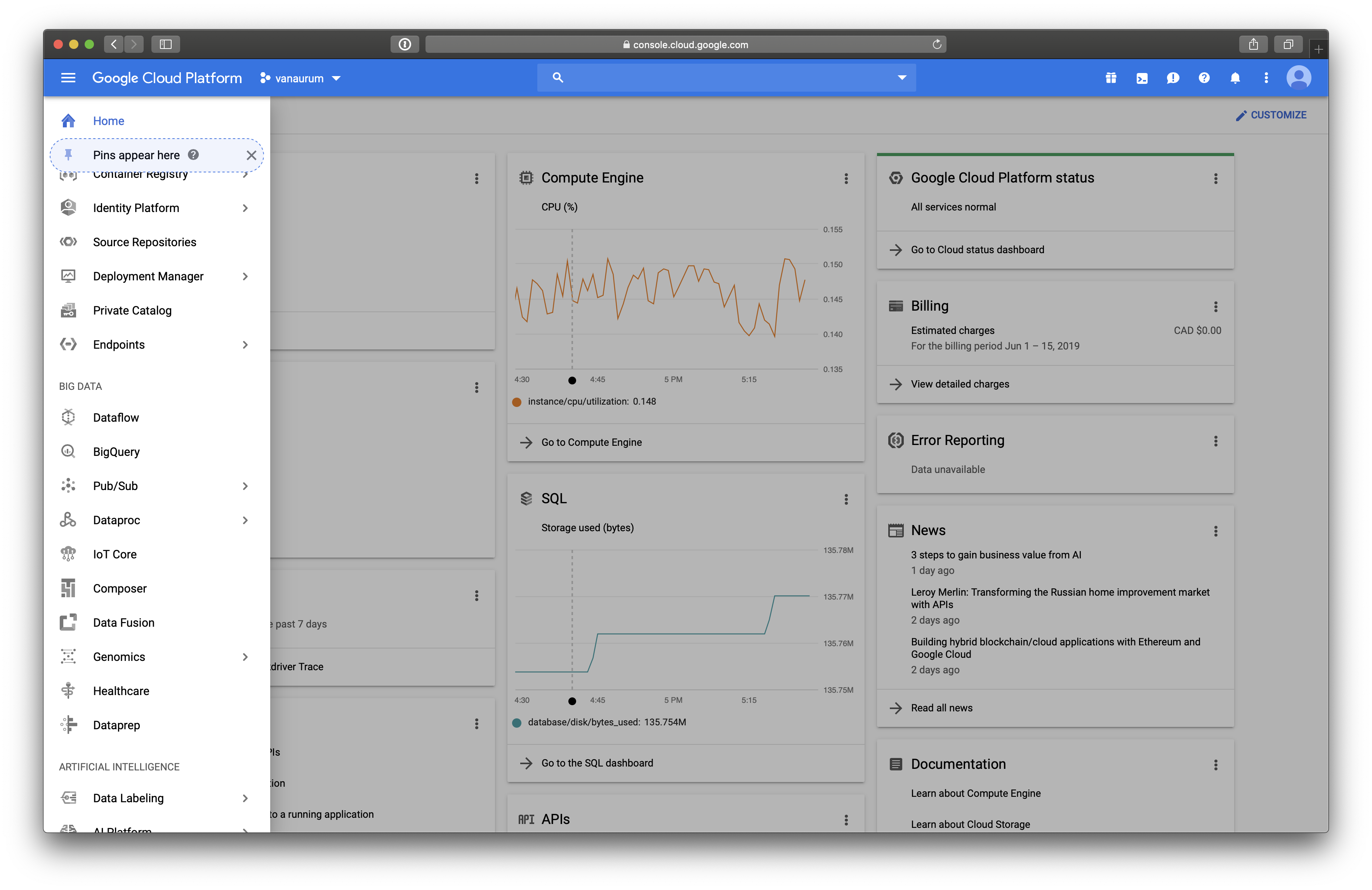
To access BigQuery ML from your google cloud console, you’ll need to navigate to the Big Data section in the Navigation menu. From there, click Big Query.

process

From here, the next thing we’re going to do is add the Google Analytics E-Commerce dataset. This dataset is pretty awesome because it contains real-world analytics data for Google’s Merchance Store. The dataset contains real-world flaws and requires real-world processes to process and clean the data before training - which we’re going to do!

Once you have the BigQuery interface open you can click this link to automatically pin the dataset to your own console.

Because this is Google Analytics data, there is awesome documentation for all the columns names here: Google Analytics Schema. You should open this in a new tab and keep it open because we’ll reference it several times in this article.

Exploratory Analysis: What Percentage of Visitors Made a Purchase?

You should see the Data-to-Insights data resource in the menu on the left. It should look something like this…

process

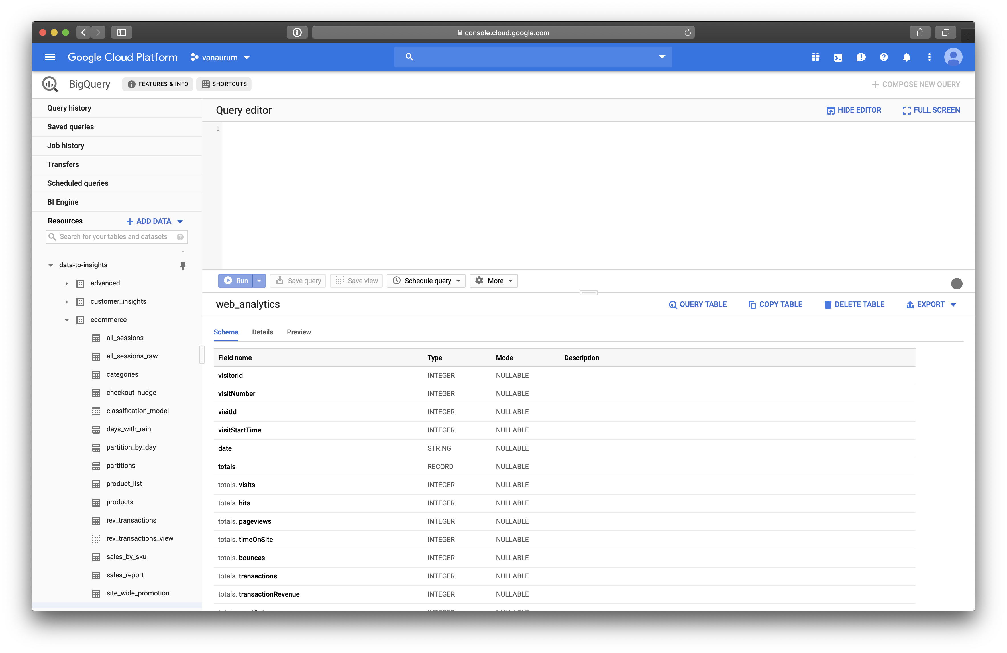
We’re going to use the web-analytics table to perform this analysis.

Quick Tip: When you have a dataset open you can click on Query_Table and it will populate the query editory with the proper table reference data. For the web_analytics table you’ll see this appear:

SELECT  FROM `data-to-insights.ecommerce.web_analytics` LIMIT 1000

To find out the percentage of visitors that made a purchase, we can use the following query.

# standardSQL
WITH visitors AS(
SELECT
COUNT(DISTINCT fullVisitorId) AS total_visitors
FROM `data-to-insights.ecommerce.web_analytics`
),

purchasers AS(
SELECT
COUNT(DISTINCT fullVisitorId) AS total_purchasers
FROM `data-to-insights.ecommerce.web_analytics`
WHERE totals.transactions IS NOT NULL
)

SELECT
  total_visitors,
  total_purchasers,
  (total_purchasers / total_visitors) *100 AS conversion_rate
FROM visitors, purchasers

Breaking Down This Query:

The WITH clause contains one or more named subqueries which execute every time a subsequent SELECT statement references them. Any clause or subquery can reference subqueries you define in the WITH clause. This includes any SELECT statements on either side of a set operator, such as UNION.

We use this primarily for readability. Here we declare two main queries: visitors and purchasers.

The visitors query pulls all the unique fullVisitorId’s from the web_analytics tables and saves it as the alias total_visitors.
The purchasers query is the same query as visitors, except it filters it for rows where a transaction has taken place.
We then calculate conversion_rate as total_purchasers / total_visitors.

Click Run Query, and you should see a result like this:

process

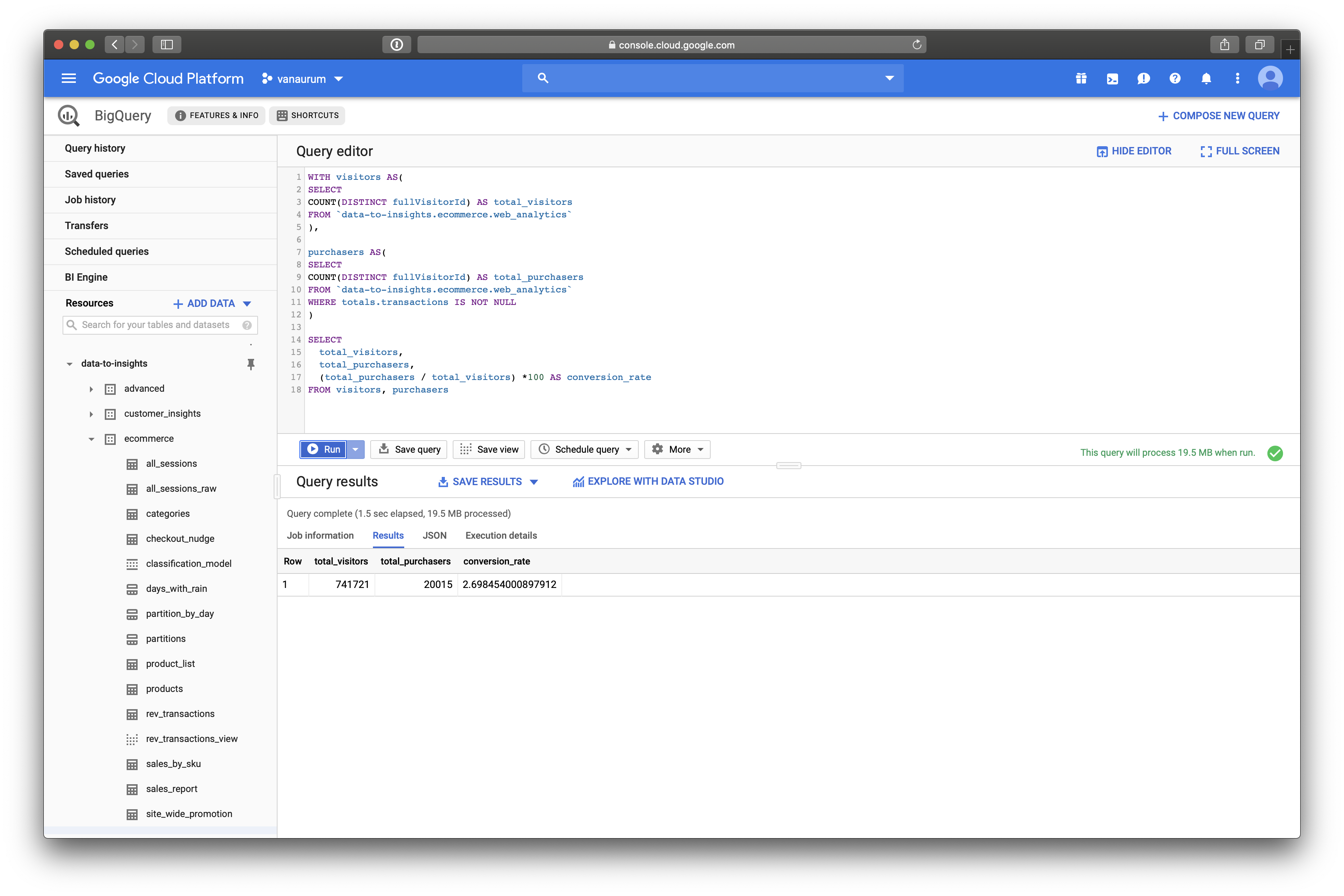
We can see that the conversation rate on visitors to Google’s Merchandise store is 2.69% from 741,721 total visitors.

Exploratory Analysis: Top and Bottom Products by Sales

Another thing this data permits us to do is find the best selling products, and worst selling products in Google’s Merchandise Store. To so this, we can run a query like the following:

# Top products
SELECT
  p.v2ProductName,
  p.v2ProductCategory,
  SUM(p.productQuantity) AS units_sold,
  ROUND(SUM(p.localProductRevenue/1000000),2) AS revenue
FROM `data-to-insights.ecommerce.web_analytics`,
UNNEST(hits) AS h,
UNNEST(h.product) AS p
GROUP BY 1, 2
ORDER BY revenue DESC
LIMIT 5;

Breaking Down This Query:

You’ll probably notice the UNNEST command here. The UNNEST command takes an array type entry and converts it into a table. If you visit the Google Analytics Schema that we referenced before, you can see why these start to make sense.

This data has a RECORD entry for hits. You’ll notice that in the schema there are sub-entries below hits, like:

hits.experiment
hits.datasource
hits.product
etc…

hits itself is an array of fields represented by hits.<subfield>. Calling the following command:

UNNEST(hits) AS h

Converts this array into a table, and saves it as h. Right after this we have another command:

UNNEST(h.product) AS p

This is because each hits.<subfield> is broken down further into hits.<subfield>.<deeper_subfield>. So to access these we need to unpack that array into a table as well and call it p. Make sense? These are just nested entries that are stored as arrays in the parent table that we need to unpack to access.

The next line…

GROUPBY 1, 2

Just means to group by the first and second column of the resulting table regardless of their names. We could also have written:

GROUPBY p.v2ProductName, p.v2ProductCategory

And gotten the same results. The results should look like this:

top_sellers

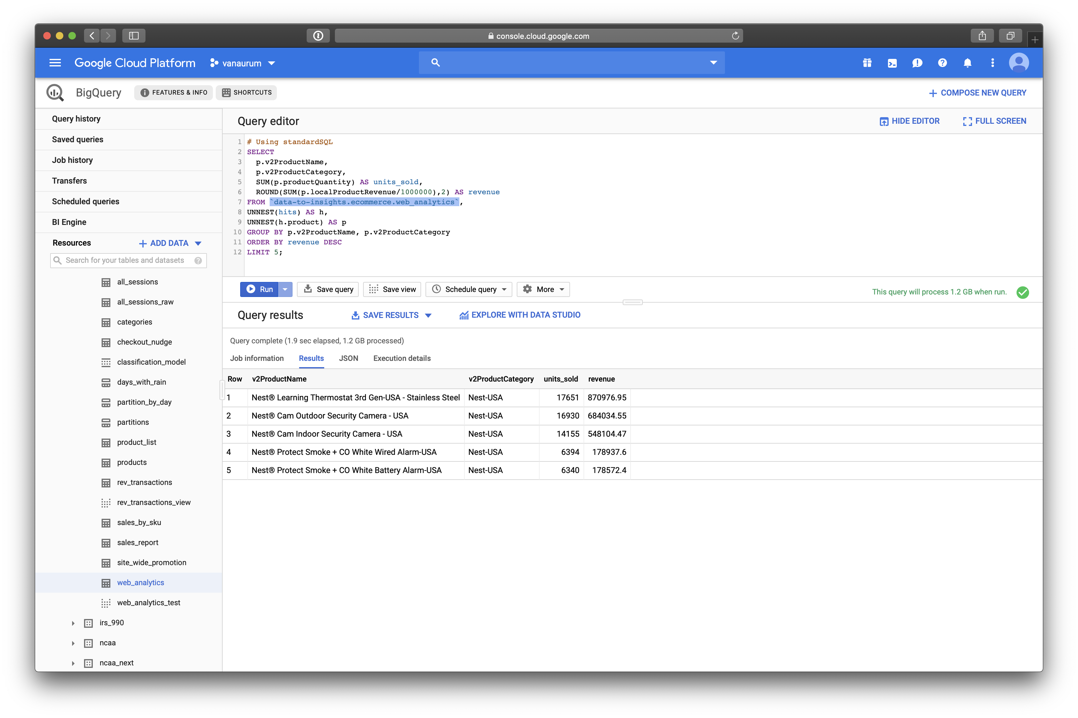
We can see that the top selling products on Google’s Merchandise Store are:

Nest® Learning Thermostat 3rd Gen-USA - Stainless Steel
Nest® Cam Outdoor Security Camera - USA
Nest® Cam Indoor Security Camera - USA
Nest® Protect Smoke + CO White Wired Alarm-USA
Nest® Protect Smoke + CO White Battery Alarm-USA

Conversely, if we flip the DESC flag to ASC we get the worst selling products.

Google Youth Girl Tee Green
Google Men’s Microfiber 1/4 Zip Pullover Grey/Black
Google Men’s Short Sleeve Hero Tee Charcoal
YouTube Twill Cap
Android Twill Cap

Exploratory Analysis: Visitors Who Bought on a Return Visit

Suppose we want to know how many visitors bought on a return visit after they had visited the site once (Whether they bought on the first visit or not)

WITH all_visitor_stats AS (
SELECT
  fullvisitorid, # Recall from first query this was 741,721 unique visitors
  IF(COUNTIF(totals.transactions > 0 AND totals.newVisits IS NULL) > 0, 1, 0) AS will_buy_on_return_visit
  FROM `data-to-insights.ecommerce.web_analytics`
  GROUP BY fullvisitorid
)

SELECT
  COUNT(DISTINCT fullvisitorid) AS total_visitors,
  will_buy_on_return_visit
FROM all_visitor_stats
GROUP BY will_buy_on_return_visit

Breaking Down This Query:

You can read this query as:

Make a query called all_visitor_stats
Retrieve columns fullvisitorid, and create a new column called will_buy_on_return_visit that:
- is 1 if the fullvisitorid has at least 1 transaction and it’s not their first time on the site.
- 0 otherwise.
Group these results bu the fullvisitorid

Note that in Google’s Schema, totals.newVisits is:

Total number of new users in session (for convenience). If this is the first visit, this value is 1, otherwise it is null.

buy_on_return

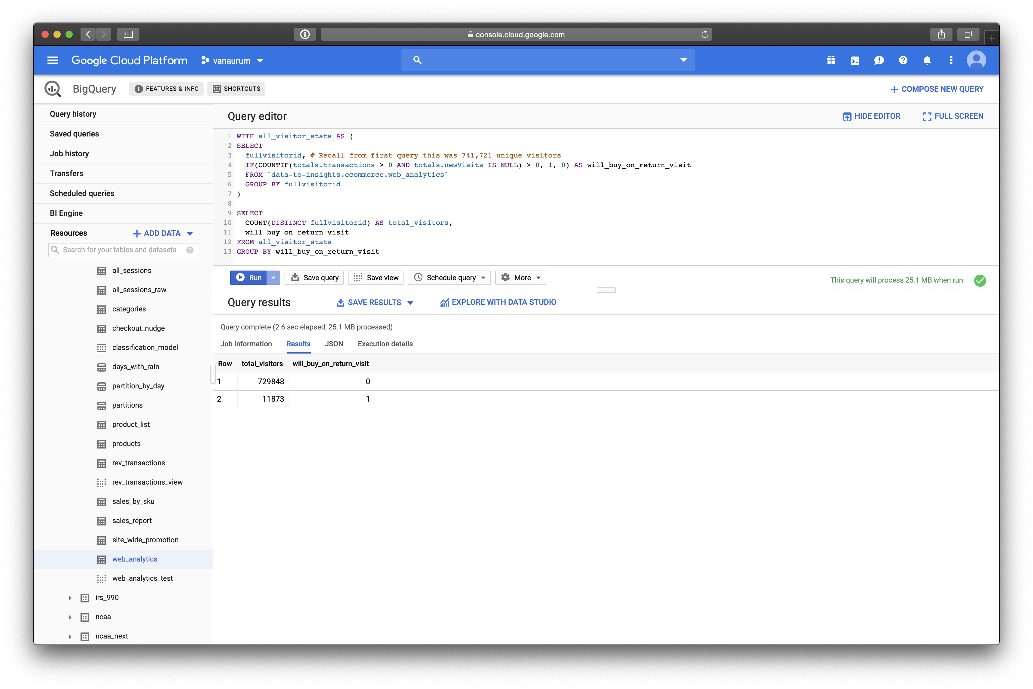
We can see that of 729,848 visitors, only 11,873 will return to make a purchase! That’s only 1.6%. Note that this includes a subset of buyers who bought the first time and also return to buy again.

Build a Machine Learning Model to Predict Future Buyers

Now we’re going to dive into the magic of Big Query ML to train a machine learning model to predict if a buyer will return in the future to make a purchase. By accurately predicting this, it can allow you to be more precise with ad-spend dollars by retargeting the visitors with this highest probability of coming back to make a purchase.

To start, we’re going to train a model on a very small subset of features and see how well the model works. This is just to get a taste of how ML models are built in BigQuery.

We’ll build our model on the following three features:

totals.pageviews: Total number of pageviews within the session.
totals.bounces: whether the visitor left the website immediately.
totals.timeOnSite: how long the visitor was on our website.

We need to assemble this data, along with our target variable that we want to predict : will_buy_on_return_visit. To do this, we’re going to create two queries and then join them:

# Take all columns excepted fullVisitorId from the following joined tables:
SELECT
  * EXCEPT(fullVisitorId)
FROM

  # Table 1
  (SELECT
    fullVisitorId,
    IFNULL(totals.bounces, 0) AS bounces,
    IFNULL(totals.timeOnSite, 0) AS time_on_site,
    IFNULL(totals.pageviews, 0) AS page_views
  FROM
    `data-to-insights.ecommerce.web_analytics`
  WHERE
    totals.newVisits = 1)
  # end of statement for table 1  

  JOIN

  # Table 2
  (SELECT
    fullvisitorid,
    IF(COUNTIF(totals.transactions > 0 AND totals.newVisits IS NULL) > 0, 1, 0) AS will_buy_on_return_visit
  FROM
      `data-to-insights.ecommerce.web_analytics`
  GROUP BY fullvisitorid)
  USING (fullVisitorId)
ORDER BY time_on_site DESC
LIMIT 10;

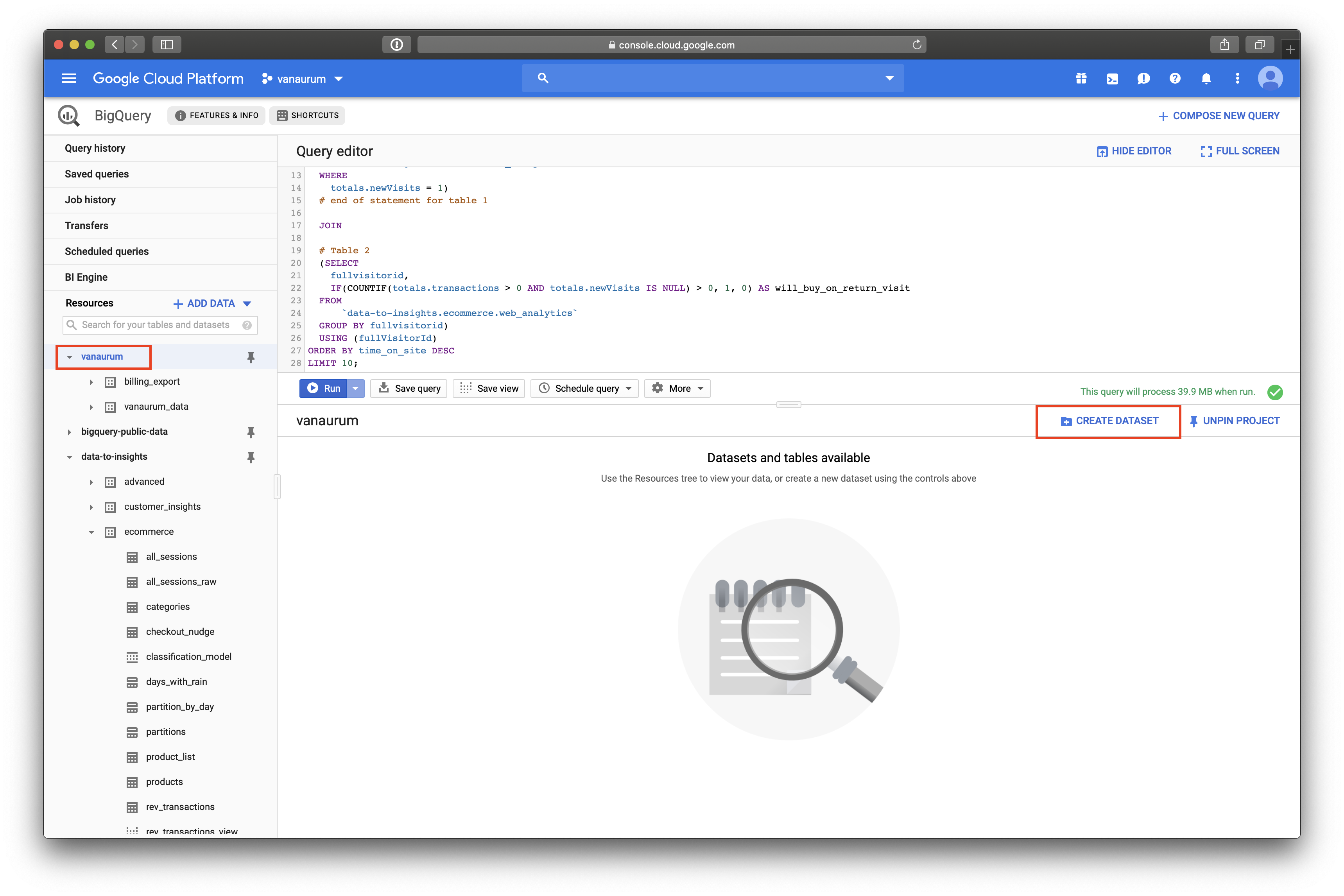
Create a BigQuery Dataset to Store ML Models

In order to store ML models, you’ll need to create a new dataset (Just like storing new data tables in your profile). To do this, click on your project name in the left pane, and then click Create Dataset.

buy_on_return

Once you create a dataset, you can write the code for the ML model. Because we’re going to be doing a classification (predicting a binary value for whether or not the visitor will return and purchase) we’re going to use logistic regression.

CREATE OR REPLACE MODEL `ecommerce.classification_model`
OPTIONS
# BigQuery ML lets you set algorithm-specifc options here
(
model_type='logistic_reg', # Declare the model we want to use
labels = ['will_buy_on_return_visit'] # Declare what our target variable is
)
AS

#standardSQL
SELECT
  * EXCEPT(fullVisitorId)
FROM

  # features
  (SELECT
    fullVisitorId,
    IFNULL(totals.bounces, 0) AS bounces,
    IFNULL(totals.timeOnSite, 0) AS time_on_site,
    IFNULL(totals.pageviews, 0) AS page_views
  FROM
    `data-to-insights.ecommerce.web_analytics`
  WHERE
    totals.newVisits = 1
    AND date BETWEEN '20160801' AND '20170430') # train on first 9 months
  JOIN
  (SELECT
    fullvisitorid,
    IF(COUNTIF(totals.transactions > 0 AND totals.newVisits IS NULL) > 0, 1, 0) AS will_buy_on_return_visit
  FROM
      `data-to-insights.ecommerce.web_analytics`
  GROUP BY fullvisitorid)
  USING (fullVisitorId)
;

Running this will take a few minutes…

When it’s done, we can explore the model’s performance parameters. BigQuery ML is actually pretty awesome in this regard - it provides analytics out of the box that give you a great sense of how well your model performs!

When the model finishes, you’ll see a Go to model button appear on the right side of the screen. Click on this. You’ll have four tabs of performance metrics to explore - click on the Evaluation tab and you’ll see the following:

buy_on_return

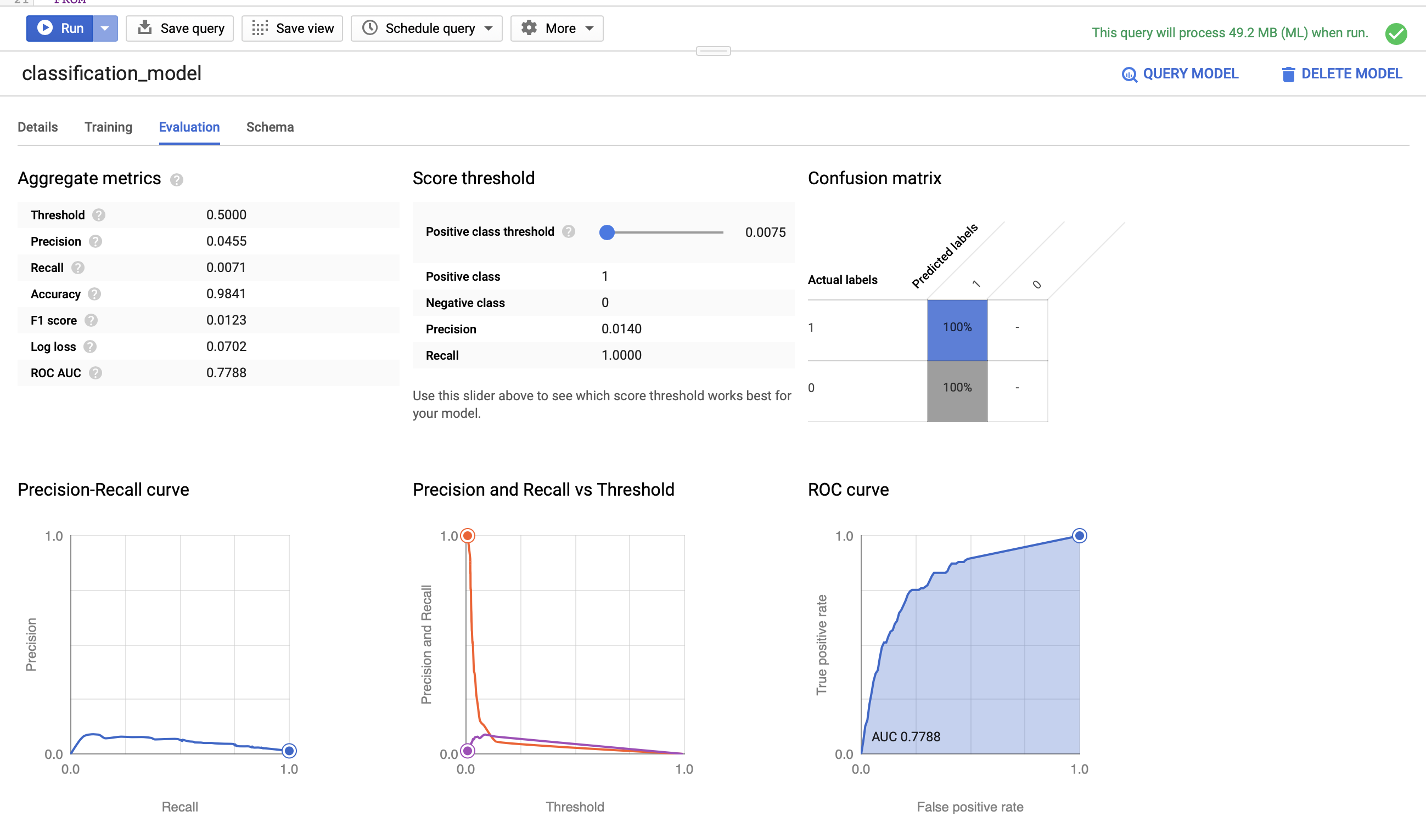
Our AUC metric is 0.7788. Let’s test the model on out-of-sample data and see how well we perform.

Evaluating the model is as simple as calling the ML.EVALUATE command on a test data query. We can do this accordingly:

SELECT
  roc_auc,
  CASE
    WHEN roc_auc > .9 THEN 'good'
    WHEN roc_auc > .8 THEN 'fair'
    WHEN roc_auc > .7 THEN 'not great'
  ELSE 'poor' END AS model_quality
FROM
  ML.EVALUATE(MODEL ecommerce.classification_model,  (

SELECT
  * EXCEPT(fullVisitorId)
FROM

  # features
  (SELECT
    fullVisitorId,
    IFNULL(totals.bounces, 0) AS bounces,
    IFNULL(totals.timeOnSite, 0) AS time_on_site,
    IFNULL(totals.pageviews, 0) AS page_views
  FROM
    `data-to-insights.ecommerce.web_analytics`
  WHERE
    totals.newVisits = 1
    AND date BETWEEN '20170501' AND '20170630') # eval on 2 months
  JOIN
  (SELECT
    fullvisitorid,
    IF(COUNTIF(totals.transactions > 0 AND totals.newVisits IS NULL) > 0, 1, 0) AS will_buy_on_return_visit
  FROM
      `data-to-insights.ecommerce.web_analytics`
  GROUP BY fullvisitorid)
  USING (fullVisitorId)

));

Here we set up thresholds for a performance column we’ll call model_quality. When we run this evaluation query, we’ll see something like this…

buy_on_return

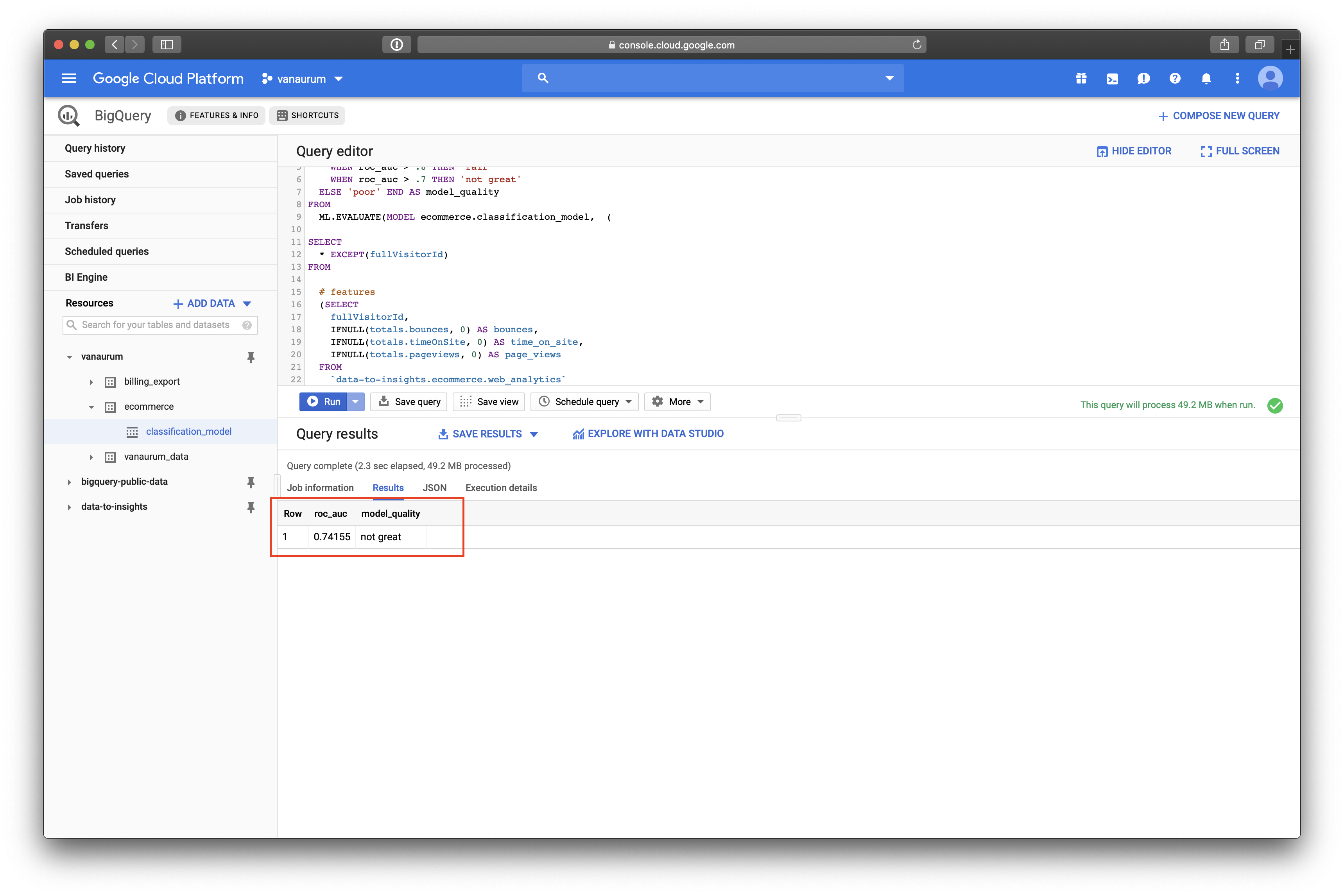
We can see that our roc_auc score for the test data was 0.74155, which equates to not_great in our scoring rubrik. Let’s see if we can beat this score by adding a richer feature set to the training data!

Improving Model Performance with Better Features

With machine learning models, the judicious addition of features can dramatically improve model performance because it gives the algorithm more dimensions from which to find structure in the data.

Perhaps there is structure hidden in the following features that can help our model (You can add any features you like here!)

How far the visitor got in the checkout process on their first visit.
Where the visitor came from (traffic source: organic search, referring site etc..)
Device category (mobile, tablet, desktop)
Geographic information (country)

Let’s create a second model called classification_model02:

CREATE OR REPLACE MODEL `ecommerce.classification_model_2`

# Same options as our first model
OPTIONS
  (model_type='logistic_reg', labels = ['will_buy_on_return_visit']) AS

WITH all_visitor_stats AS (
SELECT
  fullvisitorid,
  IF(COUNTIF(totals.transactions > 0 AND totals.newVisits IS NULL) > 0, 1, 0) AS will_buy_on_return_visit
  FROM `data-to-insights.ecommerce.web_analytics`
  GROUP BY fullvisitorid
)

# add in new features
SELECT * EXCEPT(unique_session_id) FROM (

  SELECT
      CONCAT(fullvisitorid, CAST(visitId AS STRING)) AS unique_session_id,

      # labels
      will_buy_on_return_visit,

      MAX(CAST(h.eCommerceAction.action_type AS INT64)) AS latest_ecommerce_progress,

      # behavior on the site (same set of features as before)
      IFNULL(totals.bounces, 0) AS bounces,
      IFNULL(totals.timeOnSite, 0) AS time_on_site,
      IFNULL(totals.pageviews, 0) AS page_views,
      totals.pageviews,

      # Now we add our new features: 
      # where the visitor came from
      trafficSource.source,
      trafficSource.medium,
      channelGrouping,

      # And the platform used...
      device.deviceCategory,

      # geographic
      IFNULL(geoNetwork.country, "") AS country

  FROM `data-to-insights.ecommerce.web_analytics`,
     UNNEST(hits) AS h

    JOIN all_visitor_stats USING(fullvisitorid)

  WHERE 1=1
    # only predict for new visits
    AND totals.newVisits = 1
    AND date BETWEEN '20160801' AND '20170430' # train 9 months

  GROUP BY
  unique_session_id,
  will_buy_on_return_visit,
  bounces,
  time_on_site,
  totals.pageviews,
  trafficSource.source,
  trafficSource.medium,
  channelGrouping,
  device.deviceCategory,
  country
);

Note that this line:

MAX(CAST(h.eCommerceAction.action_type AS INT64)) AS latest_ecommerce_progress

Adds the feature for how far the customer got in the checkout process. We cast this as an integer, because google defines this into levels from 1-8:

Click through of product lists = 1,
Product detail views = 2,
Add product(s) to cart = 3,
Remove product(s) from cart = 4,
Check out = 5,
Completed purchase = 6,
Refund of purchase = 7,
Checkout options = 8,
Unknown = 0.

After training, we can view this model’s performance characteristics on the training data again.

buy_on_return

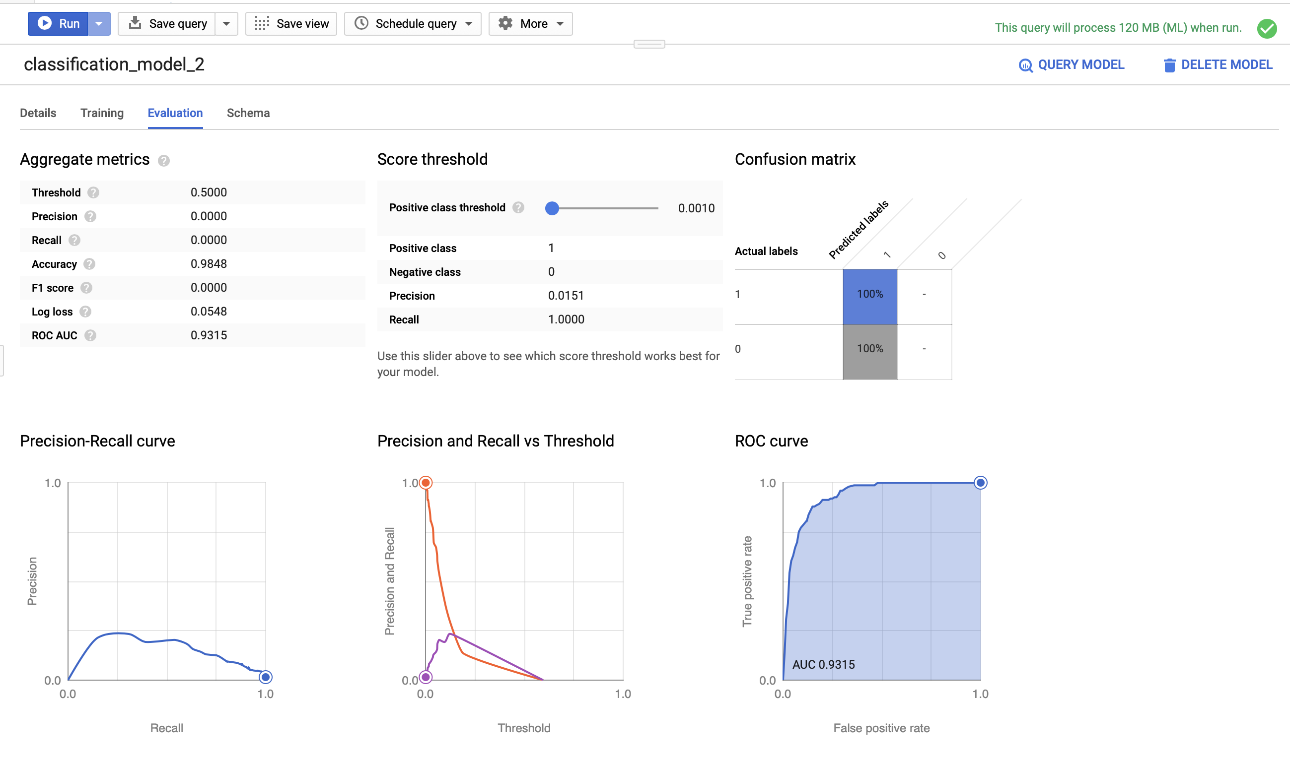
We can see that this model’s roc_auc score is 0.9315 - significantly better than our prior model with fewer features. Note that we’re training this data on the same 9 months of data as the first model so that we have an apple-to-apples comparison.

Let’s see how this model performs on the testing data. The code for building the testing set is essentially the same as the first set, with a few variables changed…

# Same model performance rubrik as before...
SELECT
  roc_auc,
  CASE
    WHEN roc_auc > .9 THEN 'good'
    WHEN roc_auc > .8 THEN 'fair'
    WHEN roc_auc > .7 THEN 'not great'
  ELSE 'poor' END AS model_quality
FROM
  # except this time we evaluate model02
  ML.EVALUATE(MODEL ecommerce.classification_model_2,  (

WITH all_visitor_stats AS (
SELECT
  fullvisitorid,
  IF(COUNTIF(totals.transactions > 0 AND totals.newVisits IS NULL) > 0, 1, 0) AS will_buy_on_return_visit
  FROM `data-to-insights.ecommerce.web_analytics`
  GROUP BY fullvisitorid
)

# add in new features
SELECT * EXCEPT(unique_session_id) FROM (

  SELECT
      CONCAT(fullvisitorid, CAST(visitId AS STRING)) AS unique_session_id,

      # labels
      will_buy_on_return_visit,

      MAX(CAST(h.eCommerceAction.action_type AS INT64)) AS latest_ecommerce_progress,

      # behavior on the site
      IFNULL(totals.bounces, 0) AS bounces,
      IFNULL(totals.timeOnSite, 0) AS time_on_site,
      IFNULL(totals.pageviews, 0) AS page_views,
      totals.pageviews,

      # where the visitor came from
      trafficSource.source,
      trafficSource.medium,
      channelGrouping,

      # mobile or desktop
      device.deviceCategory,

      # geographic
      IFNULL(geoNetwork.country, "") AS country

  FROM `data-to-insights.ecommerce.web_analytics`,
     UNNEST(hits) AS h

    JOIN all_visitor_stats USING(fullvisitorid)

  WHERE 1=1
    # only predict for new visits
    AND totals.newVisits = 1
    AND date BETWEEN '20170501' AND '20170630' # eval 2 months

  GROUP BY
  unique_session_id,
  will_buy_on_return_visit,
  bounces,
  time_on_site,
  totals.pageviews,
  trafficSource.source,
  trafficSource.medium,
  channelGrouping,
  device.deviceCategory,
  country
)
));

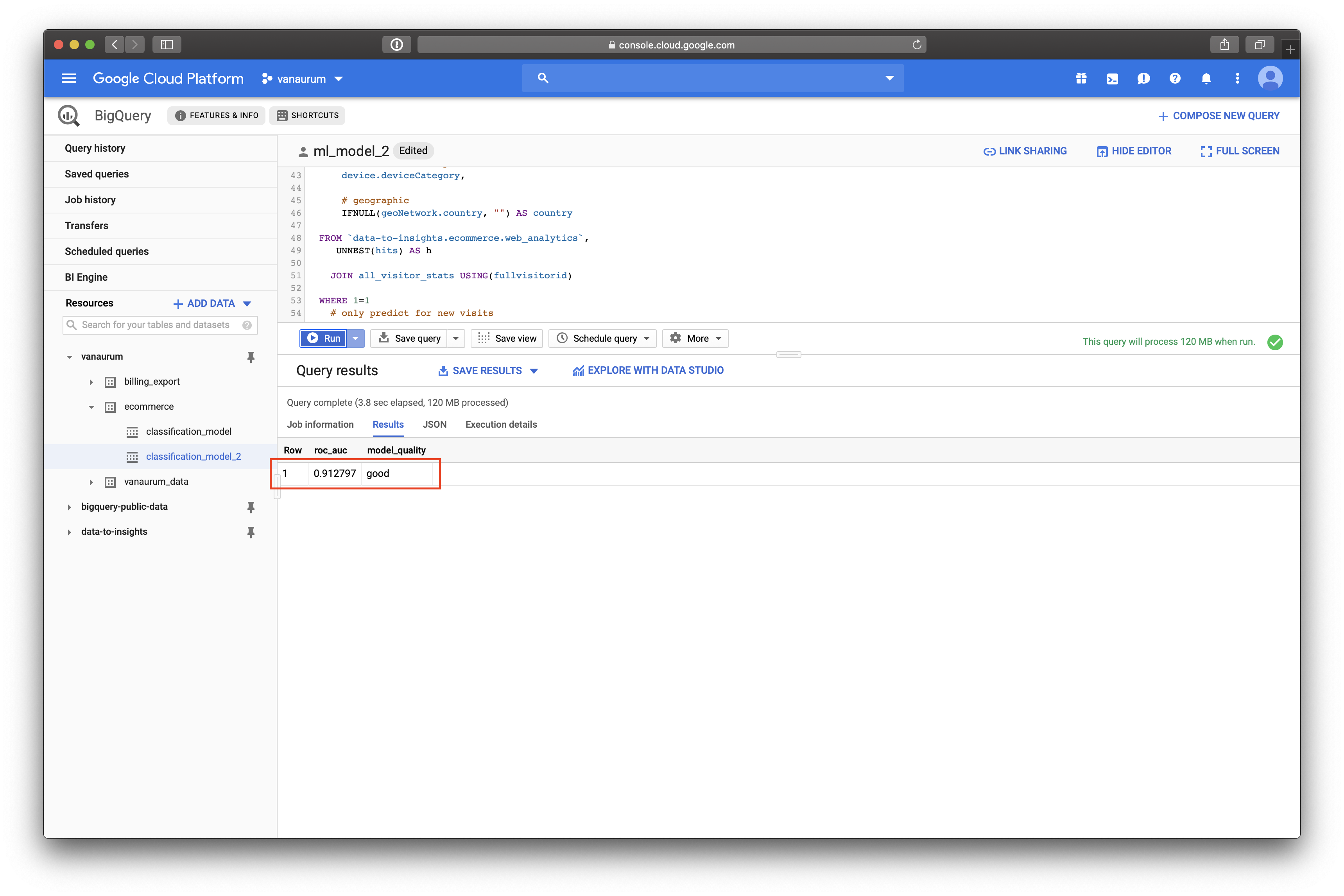
Our test set roc_auc metric is 0.912797 using this model, and our rating is good.

buy_on_return

Great! So just to recap what we have done so far:

We have created a logistic regression model to predict which new visitors will come back to the site and make a purchase.
We did this with a small set a features, and with a larger set of features.
We were able to demonstrate better roc_auc model performance with the larger set of features.

Now, to make this model even more useful we should put to work. Let’s get this model to actually tell us what new visitors have the highest probability of coming back and making a purchase.

using classification_model02, we’ll query our e-commerce dataset and return a list of new visitors ranked highest to lowest by their probability to return to the site and buy.

SELECT
*
FROM
  ml.PREDICT(MODEL `ecommerce.classification_model_2`,
   (

WITH all_visitor_stats AS (
SELECT
  fullvisitorid,
  IF(COUNTIF(totals.transactions > 0 AND totals.newVisits IS NULL) > 0, 1, 0) AS will_buy_on_return_visit
  FROM `data-to-insights.ecommerce.web_analytics`
  GROUP BY fullvisitorid
)

  SELECT
      CONCAT(fullvisitorid, '-',CAST(visitId AS STRING)) AS unique_session_id,

      # labels
      will_buy_on_return_visit,

      MAX(CAST(h.eCommerceAction.action_type AS INT64)) AS latest_ecommerce_progress,

      # behavior on the site
      IFNULL(totals.bounces, 0) AS bounces,
      IFNULL(totals.timeOnSite, 0) AS time_on_site,
      IFNULL(totals.pageviews, 0) AS page_views,
      totals.pageviews,

      # where the visitor came from
      trafficSource.source,
      trafficSource.medium,
      channelGrouping,

      # mobile or desktop
      device.deviceCategory,

      # geographic
      IFNULL(geoNetwork.country, "") AS country

  FROM `data-to-insights.ecommerce.web_analytics`,
     UNNEST(hits) AS h

    JOIN all_visitor_stats USING(fullvisitorid)

  WHERE
    # only predict for new visits
    totals.newVisits = 1
    AND date BETWEEN '20170701' AND '20170801' # test 1 month

  GROUP BY
  unique_session_id,
  will_buy_on_return_visit,
  bounces,
  time_on_site,
  totals.pageviews,
  trafficSource.source,
  trafficSource.medium,
  channelGrouping,
  device.deviceCategory,
  country
)

)

ORDER BY
  predicted_will_buy_on_return_visit DESC;

The contents of this query should be familiar by now!

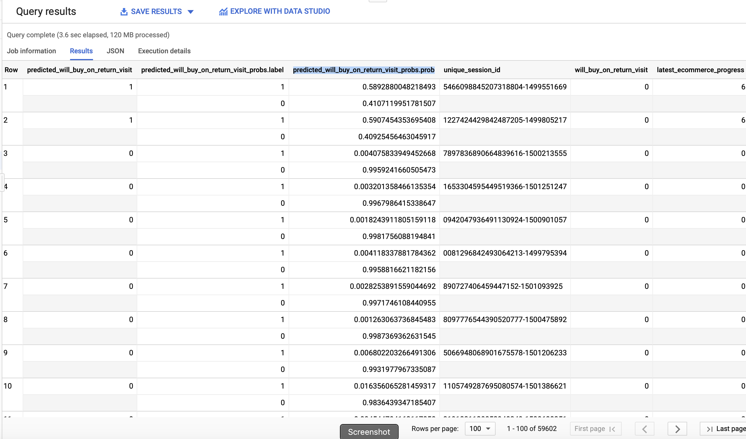
When we look at our output, we can see that BigQuery ML automatically added three new columns for us:

predicted_will_buy_on_return_visi: The ‘yes’ or ‘no’ decision from the model
predicted_will_buy_on_return_visit_probs.label: The binary classifier for yes/no
predicted_will_buy_on_return_visit_probs.prob: The confidence the model has in the prediction belonging to each label.

buy_on_return

Summary

Google BigQuery ML is a really powerful platform that leverages the parallel data processing capabilities of Big Query and integrates the ability to generate machine learning models in SQL. It allows data analysts - typically the primary user of enterprise data - to build machine learning models using a language they’re familiar with (SQL). In this post we covered the following:

Importing a dataset into Google BigQuery
Performing exploratory analysis on Google Analytics data.
Building multiple machine learning models using BigQuery ML and analyzing their performance.
Using a machine learning model to get the site visitors with the highest probability of returning to the site to buy.

If you’re confused at all by the SQL syntax used in this post, Google has an excellent documentation page on BigQuery syntax.

I hope you enjoyed this post!

In this article you will learn:

Who should read this?

Table of Contents

Introduction

Getting into the BigQuery ML Environment

Exploratory Analysis: What Percentage of Visitors Made a Purchase?

Breaking Down This Query:

Exploratory Analysis: Top and Bottom Products by Sales

Breaking Down This Query:

Exploratory Analysis: Visitors Who Bought on a Return Visit

Breaking Down This Query:

Build a Machine Learning Model to Predict Future Buyers

Create a BigQuery Dataset to Store ML Models

Improving Model Performance with Better Features

Summary