Selecting Machine Learning Algorithms Part 1
Author :: Kevin Vecmanis
In this post I demonstrate how to build a spot-checking algorithm that can evaluate a basket of machine learning algorithms on scaled and un-scaled data. By establishing a baseline performance you can then move on to forming and testing hypotheses regarding how transformations and parameter tweaks might affect your model performance.
In this article you will learn:
- How to generate a sample classification dataset
- Performing a batch spot-check on a group of algorithms
- How to build a pipeline of machine learning algorithms
- How to plot algorithm model performance
Table of Contents
- Introduction
- Creating a synthetic dataset
- Creating the test harness
- Building a test harness with a pipeline
Introduction
It’s difficult to know ahead of time what algorithm is going to work best on your dataset. Having a test harness that can spot test machine learning algorithms is a great idea - it can quickly let you know what algorithm demonstrates the most skill on your dataset out of the box. In most cases, especially with large datasets, spotchecking is limited to a single variant of the algorithm simply because of the time required to do a more thorough search of the solution space.
In this post I’m going to demonstrate how to build a spot-checking algorithm that can evaluate a basket of machine learning algorithms on scaled and un-scaled data, with integrated hypothesis testing.
We’re going to begin by creating a synthetic dataset that we can work with.
Creating a Synthetic Dataset
Sklearn has an integreated library for building sample datasets with a vareity of features. The key features are:
n_samples: The number of training samples in the dataset.n_features: The number of features (columns) in the dataset, not including the target.n_redundant: The number of features that carry no explanatory information for predicting the target class. Increase this will add noise to the training proces and make it more taxing on some of the algorthims.n_classes: The number of classes present in the target column (i.e, blue/red, cabernet/merlot). Increasing this beyond two will make it a multi-class classification problem.random_state: Seed this with a specific integer if you want the same dataset every time.
To read the complete documentation on this API visit here: sklearn.make_classification
from sklearn.datasets import make_classification
import pandas as pd
from sklearn.model_selection import train_test_split

X, Y = make_classification(n_samples = 5000,
                           n_features = 15,
                           n_informative = 2,
                           n_redundant = 10,
                           n_classes = 2,
                           random_state = 8)
Creating the Test Harness
Now that we have our training dataset, we’re going to set up a pipeline of algorithms to test. We’re going to spot-check the following algorithms in our baseline:
- Naive Bayes
- Random Forest
- Support Vector machines
- XGBoost
- KNN
- Linear Discriminant Analysis
- Logistic Regression
We’re going to use the default parameters for all of these with our baseline, with the exception of SVM which needs probability to be declared as True if you want to score using log loss.
from matplotlib import pyplot
from sklearn.ensemble import RandomForestClassifier
from sklearn.naive_bayes import GaussianNB
from sklearn.discriminant_analysis import LinearDiscriminantAnalysis
from sklearn.svm import SVC
from sklearn.neighbors import KNeighborsClassifier
from sklearn.linear_model import LogisticRegression
from sklearn.model_selection import KFold
from sklearn.model_selection import cross_val_score
from xgboost import XGBClassifier
import time
def algo_spotcheck(X,Y):
# Declare an empty list that will contain all of our pipelines.
algorithms = []
algorithms.append(['RF', RandomForestClassifier()])
algorithms.append(['NB', GaussianNB()])
algorithms.append(['LDA', LinearDiscriminantAnalysis()])
algorithms.append(['XGB', XGBClassifier()])
algorithms.append(['KNN', KNeighborsClassifier()])
algorithms.append(['SVM', SVC(probability=True)])
algorithms.append(['LOG', LogisticRegression()])
results = []
names = []
scoring = 'neg_log_loss'
start = time.time()
summary = []
# For each algorithm, test performance using 10-fold cross validation
# and log the results
for name, algo in algorithms:
kfold = KFold(n_splits=10, random_state=7)
cv_results = cross_val_score(algo, X_train, Y_train, cv=kfold, scoring = scoring)
results.append(cv_results)
names.append(name)
msg = "%s: %f (%f)" % (name, cv_results.mean(), cv_results.std())
print(msg)
summary.append([cv_results.mean(), cv_results.std(), name])
# Rank the results and display the top performer
summary = sorted(summary, reverse=True)
print('')
print ('Top performer: %s %f (%f)' % (summary[0][2], summary[0][0], summary[0][1]))
# boxplot algorithm comparison
print('')
print('Time to spot-check baseline algorithms: %.2f seconds' % (time.time() - start))
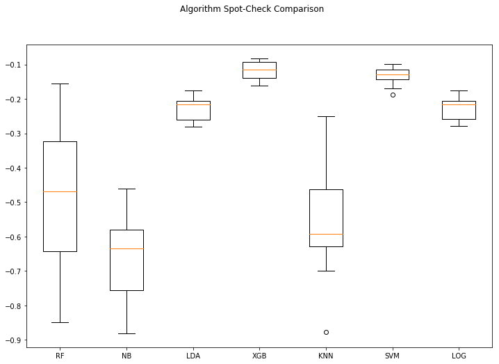
fig = pyplot.figure(figsize=(12,8))
fig.suptitle( 'Algorithm Spot-Check Comparison' )
ax = fig.add_subplot(111)
pyplot.boxplot(results)
ax.set_xticklabels(names)
pyplot.show()
returnresults = algo_spotcheck(X,Y)RF: -0.485818 (0.221462)
NB: -0.665659 (0.127054)
LDA: -0.229887 (0.033906)
XGB: -0.118912 (0.027892)
KNN: -0.563344 (0.160961)
SVM: -0.133463 (0.026566)
LOG: -0.230039 (0.033473)
Top performer: XGB -0.118912 (0.027892)
Time to spot-check baseline algorithms: 6.91 seconds
Analysis
With neg_log_loss, a score closer to zero is best. Log loss is considered to be a superior form of binary accuracy measurement because it punishes confident predictions that are wrong more than neutral predictions that are wrong.
We can see that by running our baseline algorithm spot-checking algorithm the top performing algorithm using this test harness on this dataset is XGBoost. Keep in mind that this spot-check is done without any data transformations, and only on the baseline defaults for each algorithm. It might be that we didn’t give some of the algorithms a fair shot because the data wasn’t presented properly. XGBoost doesn’t suffer performance degredation with un-scaled data like some of the other algorithms like KNN and SVM.
We can modify our spotchecking algorithm to make it more robust and give all the algorithms a fair shake. Let’s make some changes to the function we created so that it does to comparisons - one using unscaled data, and the other using scaled data. Then we can merge the results, plot, and compare.
We can leverage the Pipeline function in Python to apply a standard scaler to the data during each fold of the cross-validation process.
Building a Pipelined Test Harness
from sklearn.pipeline import Pipeline
from sklearn.preprocessing import StandardScaler

def algo_spotcheck(X,Y):

    # Declare an empty list that will contain all of our pipelines.
    algorithms=[]
    algorithms.append(['RF', RandomForestClassifier()])
    algorithms.append(['RF(s)',  Pipeline([('Scale',StandardScaler()),('RF',RandomForestClassifier())])])
    algorithms.append(['NB', GaussianNB()])
    algorithms.append(['NB(s)',  Pipeline([('Scale',StandardScaler()),('NB',GaussianNB())])])
    algorithms.append(['LDA', LinearDiscriminantAnalysis()])
    algorithms.append(['LDA(s)',  Pipeline([('Scale',StandardScaler()),('LDA',LinearDiscriminantAnalysis())])])
    algorithms.append(['XGB', XGBClassifier()])
    algorithms.append(['XGB(s)',  Pipeline([('Scale',StandardScaler()),('XGB',XGBClassifier())])])
    algorithms.append(['KNN', KNeighborsClassifier()])
    algorithms.append(['KNN(s)',  Pipeline([('Scale',StandardScaler()),('KNN',KNeighborsClassifier())])])
    algorithms.append(['SVM', SVC(probability=True)])
    algorithms.append(['SVM(s)',  Pipeline([('Scale',StandardScaler()),('SVM',SVC(probability=True))])])
    algorithms.append(['LOG', LogisticRegression()])
    algorithms.append(['LOG(s)',  Pipeline([('Scale',StandardScaler()),('LOG',LogisticRegression())])])

    results = []
    names = []
    scoring = 'neg_log_loss'
    start = time.time()
    summary = []

    #For each algorithm, test performance using 10-fold cross validation
    #and log the results
    for name, algo in algorithms:
      kfold = KFold(n_splits=10, random_state=7)
      cv_results = cross_val_score(algo, X, Y, cv=kfold, scoring=scoring)
      results.append(cv_results)
      names.append(name)
      msg = "%s: %f (%f)" % (name, cv_results.mean(), cv_results.std())
      print(msg)
      summary.append([cv_results.mean(),cv_results.std(),name])

    # Rank the results and display the top performer

    summary = sorted(summary, reverse=True)
    print('')
    print ('Top performer: %s %f (%f)' % (summary[0][2], summary[0][0], summary[0][1]))

    # Boxplot algorithm comparison

    print('')
    print('Time to spot-check baseline algorithms: %.2f seconds' % (time.time() - start))
    fig = pyplot.figure(figsize=(12,8))
    fig.suptitle( 'Algorithm Spot-Check Comparison' )
    ax = fig.add_subplot(111)
    pyplot.boxplot(results)
    ax.set_xticklabels(names)
    pyplot.show()

    return

algo_spotcheck(X, Y) (Note: (s) means scaled)
RF: -0.491498 (0.164453)
RF(s): -0.496037 (0.249087)
NB: -0.665659 (0.127054)
NB(s): -0.665659 (0.127054)
LDA: -0.229887 (0.033906)
LDA(s): -0.229887 (0.033906)
XGB: -0.118912 (0.027892)
XGB(s): -0.118912 (0.027892)
KNN: -0.563344 (0.160961)
KNN(s): -0.588833 (0.210363)
SVM: -0.133332 (0.026747)
SVM(s): -0.133592 (0.026458)
LOG: -0.230039 (0.033473)
LOG(s): -0.230036 (0.033452)
Top performer: XGB(s) -0.118912 (0.027892)
Time to spot-check baseline algorithms: 13.45 seconds
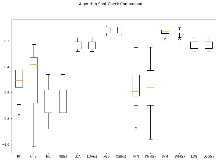
So now we have a more robust test harness that spot-checks the algorithms using scaled data and un-scaled data. Note that when a pipeline object gets passed to the cross_val function it executes the operations in the pipeline sequentially each time.
So far so good. But can we do better? Of course. The issue at hand is that each of these algorithms have hyperparameters that can be tuned. It might be the case that one of these algorithms, appropriately tuned, might exceed the performance of XGBoost. It also might be the XGBoost’s score might become even better when properly tuned.
The problem with doing this, especially on big datasets, is that you need a lot of computing power to scan the entire solution space. In part we’ll adapt these functions to incorporate intelligent search with Hyperopt.
Thanks for reading!