How to implement Bayesian Optimization in Python
Author :: Kevin Vecmanis
In this post I do a complete walk-through of implementing Bayesian hyperparameter optimization in Python. This method of hyperparameter optimization is extremely fast and effective compared to other “dumb” methods like GridSearchCV and RandomizedSearchCV.
In this article you will learn:
- What Bayesian Optimization is.
- Why you need to know it.
- How to use the hyperopt library - an implementation of this method in Python.
- How to structure your objective functions.
- How to save the Trials() object and load it later.
- How to implement it with the popular XGBoost classification algorithm.
- How to plot the Hyperopt search pattern.
Table of Contents
- Introduction: Taking people out of the loop
- What is Hyperopt
- Setting up GridSearch and RandomizedSearch
- Setting up Hyperopt for intelligent search
- The objective function
- The search space
- The fmin function
- Saving the Trials() object
- Using Hyperopt to tune XGBoost
- Visualizing Hyperopt’s Search Pattern
Introduction: Taking People Out of the Loop
If you have ever done a parameter search using GridSearchCV or RandomizedSearchCV, you understand how quickly the time requirements for these searches can explode when you want to do a comprhensive search for the best solution (search space). Bayesian Optimization is an amazing solution to this problem, and offers a more ‘intelligent’ search strategy.
Bayesian Optimization works building a probability-based model, sequentially, and adjusting that model after each iteration. There is a lot of research on this optimization method available, but in this post we’re going to focus on the practical implementation in Python.
You can read a paper on Bayesian Optimization here: Link to Bayesian Optimization paper
Bayesian Optimization is a must have tool in a data scientist’s tool kit - simply because it outperforms other methods of parameter search dramatically.
Throughout the rest of the article we’re going to introduct the Hyperopt library - a fantastic implementation of Bayesian Optimization in Python - and use to to compare algorithm performance against grid search and randomized search.
Hyperopt
Hyperopt is a Python implementation of Bayesian Optimization. Throughout this article we’re going to use it as our implementation tool for executing these methods. I highly recommend this library!
Hyperopt requires a few pieces of input in order to function:
- An objective function
- A Parameter search space
- The hyperopt minimization function
I’m going to walk through how to build each of these, but first let’s assemble our toy dataset.
from sklearn.datasets import make_classification
import pandas as pd

X,Y=make_classification(n_samples=300,
                        n_features=25,
                        n_informative=2,
                        n_redundant=10,
                        n_classes=2,
                        random_state=8)
The next thing we’re going to do is set up an implementation of GridSearchCV and RandomizedSearchCV so that we can compare their performance on this dataset to Hyperopt.
Note: To use hyperopt you’ll need to open a terminal and run:
$ pip install hyperopt
Setting up GridSearch and RandomizedSearch
from sklearn.model_selection import KFold
from sklearn.model_selection import cross_val_score
from sklearn.grid_search import GridSearchCV
from sklearn.grid_search import RandomizedSearchCV
import time
import numpy as np

classifier = SVC()
metric = 'neg_log_loss'

#Parameter search space for both GridSearch and RandomizedSearch
params={
        'C': np.arange(0.005,1.0,0.005),
        'kernel': ['linear', 'poly', 'rbf'],
        'degree': [2,3,4],
        'probability':[True]
        }

n_iter = 200
random_search = RandomizedSearchCV(classifier,
                                   param_distributions = params,
                                   n_iter = n_iter,
                                   scoring = metric)

# Run the fit and time it
start = time.time()
random_search.fit(X,Y)
elapsed_time_random = time.time() - start

grid_search = GridSearchCV(classifier,
                           param_grid = params,
                           scoring = metric)

start = time.time()
grid_search.fit(X,Y)
elapsed_time_grid = time.time() - start

print("GridSearchCV took %.2f seconds" % (elapsed_time_grid)
print(grid_search.best_score_, grid_search.best_params_)

print("RandomizedSearchCV took %.2f seconds for %d candidates" % (elapsed_time_random, n_iter))
print(random_search.best_score_, random_search.best_params_)
RandomizedSearchCV took 5.57 seconds for 200 candidates
-0.3025122527046663 {'probability': True, 'kernel': 'rbf', 'degree': 4, 'C': 0.85}
GridSearchCV took 43.80 seconds
-0.298021975049231 {'C': 0.975, 'degree': 4, 'kernel': 'rbf', 'probability': True}
Setting up Hyperopt for Intelligent Search
For Hyperopt, we have to define a function that the hyoperopt ‘Tree of Parzen Estimators’ (TPE) algorithm will seek to minimize, as well as a new search space that’s in the appropriate format for the hyperopt algorithm. Our GridsearchCV and RandomizedSearchCV defaulted to 3-Fold cross validation so we will replicate that in our objective function.
Because the natural tendency of fmin is to minimize the score from the objective function, we’ll multiply our cross_val_score by negative 1 to make it positive. Take caution to assess this on a case-by-case basis. Here we’re using neg_log_loss as a scoring function. Lower absolute log loss scores are ideal, so we need to multiple this score by -1 to make it a positive integer. If we didn’t, Hyperopt would seek to make the neg_log_loss value more and more negative which would increase the absolute log loss value!
We define one new function: An objective function with output that we seek to minimize.
The Objective Function
best_score=1.0

def objective(space):

    global best_score
    model = SVC(**space)
    kfold = KFold(n_splits=3, random_state=1985, shuffle=True)
    score = -cross_val_score(model, X, Y, cv=kfold, scoring=metric, verbose=False).mean()

    if (score < best_score):
        best_score=score

    return score
The Search Space
Hyperopt needs a search space from which to sample and select hyperparameters. The search space will be different for each algorithm that you work with. Here is our search space for SVC which captures most of the main hyperparameters. Note that you can add more parameters to this if you wish.
from hyperopt import hp, fmin, tpe, rand, STATUS_OK, Trials

space = {
      'C': hp.choice('x_C', np.arange(0.005,1.0,0.005)),
      'kernel': hp.choice('x_kernel',['linear', 'poly', 'rbf']),
      'degree':hp.choice('x_degree',[2,3,4]),
      'probability':hp.choice('x_probability',[True])
      }
The fmin function
The last piece of the equation is Hyperopt’s fmin function, which will take the following arguments:
- Our
objectivefunction which produces the value Hyperopt attempts to minimize. - A sample of our search
space algo: denotes the algorithm to use to build the bayesian model.max_evals: The number of sequential iterations to run (number of search space samples to test)Trials(): The trials objective is an interesting feature because it allows you to store the progress of the bayesian and then pick-up where you left off at a later time.
start = time.time()
best = fmin(
  objective,
  space = space,
  algo = tpe.suggest,
  max_evals = 25,
  trials = Trials(),
  )

print("Hyperopt search took %.2f seconds for 200 candidates" % ((time.time() - start)))
print(-best_score, best)
Hyperopt search took 1.89 seconds for 25 candidates
-0.2869846539767595 {'C': 193, 'x_degree': 1, 'x_kernel': 2, 'x_probability': 0}
Saving the Trials() Object
The Trials() object can be stored using pickle and then reloaded later like this:
import pickle
pickle.dump(trials, open("trials.p", "wb"))
trials = pickle.load(open("trials.p", "rb")) # Pass this to Hyperopt during the next training run.
Note that hyperopt was only permitted to run 25 trials, and found a better score than both GridSearchCV and RandomizedSearchCV which each used 200 trials.
Now that we have an introduction to Hyperopt, let’s do another example - this time using XGBoost.
Using Hyperopt to tune XGBoost
Let’s use the same toy dataset and see if we can get XGBoost to beat our baseline score of -0.28698 achieved previously.
Our code is going to look like this - these pieces should be familiar to you by now!
from xgboost import XGBClassifier

# Declare xgboost search space for Hyperopt
xgboost_space={
            'max_depth': hp.choice('x_max_depth',[2,3,4,5,6]),
            'min_child_weight':hp.choice('x_min_child_weight',np.round(np.arange(0.0,0.2,0.01),5)),
            'learning_rate':hp.choice('x_learning_rate',np.round(np.arange(0.005,0.3,0.01),5)),
            'subsample':hp.choice('x_subsample',np.round(np.arange(0.1,1.0,0.05),5)),
            'colsample_bylevel':hp.choice('x_colsample_bylevel',np.round(np.arange(0.1,1.0,0.05),5)),
            'colsample_bytree':hp.choice('x_colsample_bytree',np.round(np.arange(0.1,1.0,0.05),5)),
            'n_estimators':hp.choice('x_n_estimators',np.arange(25,100,5))
            }

best_score = 1.0

def objective(space):

    model = XGBClassifier(**space, n_jobs=-1)
    kfold = KFold(n_splits=3, random_state=1985, shuffle=True)
    score = -cross_val_score(model, X, Y, cv=kfold, scoring='neg_log_loss', verbose=False).mean()

    if (score < best_score):
        best_score = score

    return score

start = time.time()

best = fmin(
  objective,
  space = xgboost_space,
  algo = tpe.suggest,
  max_evals = 200,
  trials = Trials())

print("Hyperopt search took %.2f seconds for 200 candidates" % ((time.time() - start)))
print("Best score: %.2f " % (-best_score))
Print("Best space: ", best)
Hyperopt search took 28.61 seconds for 200 candidates
Best score: -0.21250464306833847
Best space: {'x_colsample_bylevel': 11, 'x_colsample_bytree': 5, 'x_learning_rate': 13, 'x_max_depth': 1, 'x_min_child_weight': 8, 'x_n_estimators': 6, 'x_subsample': 11}
We can see that given 200 trials, Hyperopt was able to get XGBoost to produce a score that outperformed our previous baseline.
Visualizing Hyperopt’s Search Pattern
Next we’re going to modify our function a little bit to capture the history of the scores versus time so we can get a visual of what Hyperopt is doing.
import matplotlib.pyplot as plt

score_history = []
best_score_history = []

def objective(space):

    model = XGBClassifier(**space, n_jobs=-1)
    kfold = KFold(n_splits=3, random_state=1985, shuffle=True)
    score = -cross_val_score(model, X, Y, cv=kfold, scoring='neg_log_loss', verbose=False).mean()

    if (score < best_score):
        best_score=score

    best_score_history.append(best_score)
    score_history.append(score)
    return score

start=time.time()

fmin(
  objective,
  space = xgboost_space,
  algo = tpe.suggest,
  max_evals = 200,
  trials = Trials(),
  )

Y = score_history
X = list(range(1, 201, 1))
plt.figure(figsize=(10,8))
plt.xlabel('Iteration')
plt.ylabel('Log_loss')
plt.title('Hyperopt Search Pattern')
plt.plot(X, Y, 'ro')
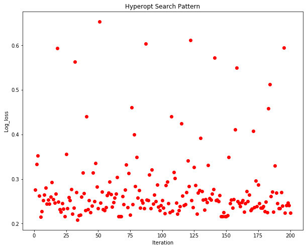
The search pattern of Hyperopt is interesting. We can see that as the number of iterations progress, the algorithm attempts new permutations of the hyper parameters and then converges them quickly back to a minima.
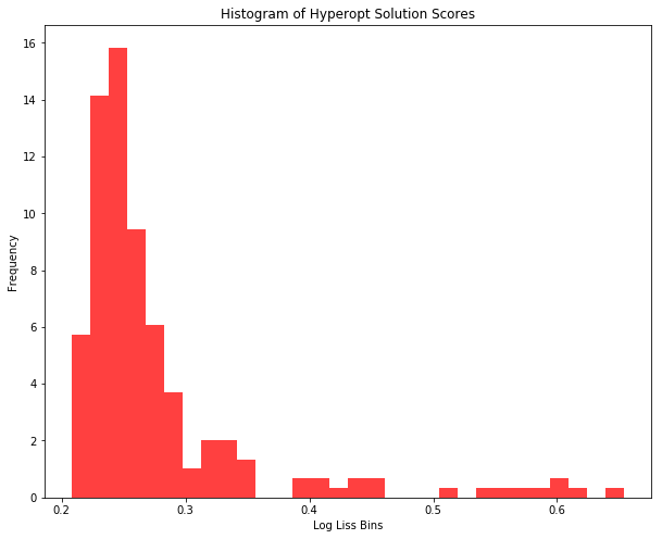
We can also plot a histogram of these results to see where the score cluster.
plt.figure(figsize = (10,8))
plt.xlabel('Log Liss Bins')
plt.ylabel('Frequency')
plt.title('Histogram of Hyperopt Solution Scores')
plt.hist(Y, 30, density=True, facecolor='r', alpha=0.75)
plt.show
Summary
- Compared to
GridSearchCVandRandomizedSearchCV, Bayesian Optimization is a superior tuning approach that produces better results in less time. - With
hyperopt, the trial history can be saved and the training process continued by reloading theTrials()object. Hyperoptrequires the creation of a custom search space and objective function.- Bayesian optimization is an essential tool for any machine learning engineer or data scientist!
I hope you enjoyed this article!