An Intuitive Walk-through of Linear Regression in Python

Apr 5, 2019
Author :: Kevin Vecmanis

In this article I do my best to explain some of the more confusing regression-related topics using something that we can all relate to - pizza! Through the course of the tutorial, I introduce regressions, the intuition behind them, how to execute them in Python, and how to interpret the results.

In this article you will learn:

• The intuition behind regressions
• Multiple regressions in Python
• How to interpret the results of a regression analysis
• Principles of misspecification
• Collinearity, heteroscedasticity, autocorrelation and other data issues that can affect regression results.

Table of Contents

• The intuition behind regressions
• Ranking pizza using multiple regression
• Creating our Pizza Score dataset using Sklearn
• Running the regression
• Interpreting the results
• Visualzing the important factors
• Principles of Model Specification
• Collinearity, heteroscedasticity, and serial correlation

The Intuition Behind Regressions

First, let’s clear up some terms and get an intuitive understanding of what these things are. When I studied engineering at school I was always frustrated with the professors’ inability to explain things intuitively. They weren’t all bad at it - some of the best professors I had would dedicate half of a class to conceptualizing things first (intuitively), and then spend the remainder of the class diving into the math. I think this is a great way to present complex subjects - concepts first, math later.

The key thing to remember with regressions is that we use them to explain one thing using other things.

What does this mean? Well, in science we can say that most phonomena are a function of other things. Newton discovered that force is a function of mass and acceleration. The electrical current running through a conducting wire is a function of the voltage applied and the resistance of the wire. We can also say that these things, force and current, are very well described by these correpsonding variables. That is, their ability to explain these variables is good enough that any error in the explanation is negligible or manageable.

Most things are complex, and we need multiple explanatory variables to describe them. Imagine you sit down at a wine tasting and you’re asked to describe the flavour of five different wines. Imagine further that you’re only allowed to describe them according to their acidity. That definitely restrains things, doesn’t it? Wines can definitely be described in terms of their acidity, but to truly explain them more variables are required. Wine is a complex chemical compound and some people dedicate their entire lives to understanding it. Another important concept here is that things can be explained to varying degrees.

This is the key difference between what’s called a simple linear regression, and the broader class of regressions called multiple regressions. Simple linear regressions are used when one variable adequately describes another. Multiple regressions are used when multiple variables are required to adequately describe a phenomenon. As you can imagine, most things in the world are reasonably complex in nature - and this is why multiple regression is most often used.

Getting slightly more technical now…

To tighten up this intuition a bit, let’s work on the language. Now that we know regressions are used to explain one thing using one or more variables - like the flavour of a wine - what’s actually taking place?

What we’re actually doing, mathematically, is taking a weighted combination of one or more independent variables that explain the variability of the dependent variable. The generalized equation of multiple regressions is the following:

\(Y_i = B_0 + B_1 X_1i + ... + B_k X_ki + \epsilon\)

• The variable on the left side of the equation, \(Y_i\) , is the dependent variable.
• The variables \(X_i1\) are the independent variables
• The variables \(B_k\) are the weights corresponding to each independent variable
• \(\epsilon_i\) is an error term (Because nothing can be perfectly described in the real world)

Ranking pizza using multiple regression

The equation above can be intimidating if you’re new to multiple regressions. Let’s use an example here to conceptually explain this and make it a little more intuitive - Pizza (my personal favourite!).

Suppose I want to rank my own favourite pizza on a scale of 1 to 10. Suppose further that I have been collected data on all the pizzas that I have eaten and ranking them with corresponding attributes.

This isn’t overly scientific, but it will serve the example well. Now, people have different preferences for how they like their pizza - suppose we have some variables that explain how likely I am to like a pizza. These are the attributes that I have been using to rank my theoretical pizza consumption.

• Crust thickness (Thickness)
• Crust crispness (Crisp)
• Amount of sauce per square inch of pizza (SPSI)
• Amount of cheese per square inch (CPSI)

We can re-write our regression equation to look something like this:

\(PizzaScore = B_0 + B_1 Thickness + B_2 Crisp + B_3 SPSI + B_4 CPSI + \epsilon\)

What does this mean? Well, it means that the score I give a pizza will be explained - hopefully, and at least partially - by a weighted combination of the thickness, crisp, amount of sauce, and the amount of cheese.

Our \(B_i\) factors are weights - because some of these factors might be more important than others. Perhaps the amount of sauce on my pizza isn’t as important to me as the amount of cheese - the weights for each independent variable will account for this.

\(\epsilon\) is the error term, because there is likely some variability in this equation (it is , after all, very subjective) that won’t be accounted for in the variables.

The term \(B_0\) is a constant factor. In this case, maybe I really love pizza, and no matter what I’m always going to give the score a 3 out of 10 because I like pizza so much. This factor always represents the portion of the dependent variable that doesn’t depend on the independent variables (thickness, crisp, etc…).

You will see this constant factor in every regression - and it can be very important. A lot of advanced investing strategies actually rely on “hedging” out all of the other independent variables so that you’re only left with this constant.

What if other things affect how much I like pizza?

A key take-away here with multiple regressions is that in most situations we won’t be able to perfectly describe the dependent variable - in this case the Pizza Score. There may be other factors that affect the score - like how long the pizza has sat in the box, the number of toppings on it, the type of cheese being used, the acidity or sweetness of the sauce (or any number of other tangible factors you might be able to think of). There may even be intangible factors like how hungry you are when you eat the pizza.

This is actually a fundamental problem in data science and machine learning - we call this feature engineering. Feature engineering is the creation of quantifiable data points that can improve regressions or other predictive models. I’m not going to go too deep on that here - but keep that in mind. Later, when we talk about the coefficient of determination you’ll see why these lack of variables can affect a regression.

Hopefully this gives you an intuitive grasp of what we’re trying to achieve with regression. Now we’re going to dive deeper.

Creating our Pizza Score dataset using Sklearn

The first thing we’re going to do is import the libraries we need, and create our toy dataset using SKLearn’s handy dataset creation library. The datasets library allows you to create test datasets with a lot of control and flexibility. We mentioned above that our regression is going to have four variables (THICKNESS, CRISP, SPSI, and CPSI), and one dependent variable (Pizza Score).

We’re going to call our four variables, collectively, “pizza_features”, and our dependent variable “pizza_score”. Using the make_regression function, we’ll create a dataset with the following features:

• 1000 samples. This would mean I ate and scored 1000 pizzas (which I could easily do, by the way!)
• Our number of features, n_features, is 4 (thickness, crisp, SPSI, and CPSI)
• I’m going to set the number of informative features to 2. This means only two of our four pizza attributes will end up being important to the Pizza Score. We could set this to whatever we want, but to demonstrate some of the concepts behind the regression we’re going to leave these “useless” variables in.

I seed the random number generator in numpy so that if I have to rerun this notebook the same dataset will be generated.

import numpy as np
from sklearn.datasets import make_regression
from sklearn.preprocessing import MinMaxScaler
import pandas as pd
import matplotlib.pyplot as plt
import statsmodels.api as sm
import statsmodels.formula.api as smf

np.set_printoptions(precision=2)
np.random.seed(813)
pizza_features, pizza_score = make_regression(
    n_samples = 1000, # number of samples
    n_features = 4,   # number of pizza attributes (Thickness, crisp, etc...)
    n_informative = 2 # The number of attributes that are actually going to matter for our model
)

Scale the Pizza Score

print (max(pizza_score))
print (min(pizza_score))

74.43087414338704
-83.54014698616761

We can easily scale this data so that it’s between 0 and 1, and then multiple the entire array by 10. We can then confirm that our pizzas scores are all contained with 0 and 10.

pizza_score=(pizza_score-min(pizza_score))/(max(pizza_score)-min(pizza_score))*10
print (max(pizza_score))
print (min(pizza_score))

10.0
0.0

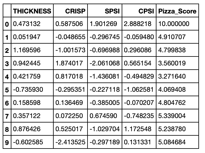
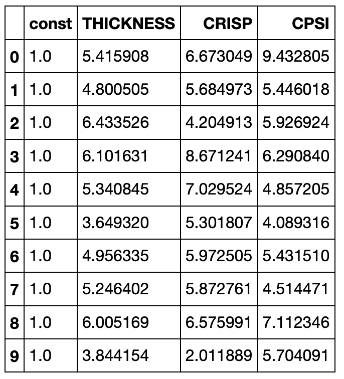
Just for fun, we can combine both entries into a single dataframe so that we can see our pizza scores alongside all of the attributes…

pizza_attributes = ['THICKNESS','CRISP','SPSI','CPSI']
pizza_features_df = pd.DataFrame(pizza_features, columns=pizza_attributes)
pizza_score_df = pd.DataFrame(pizza_score,columns=['Pizza_Score'])
pizza_df = pizza_features_df.merge(pizza_score_df, left_index=True, right_index=True)
pizza_df.head(10)

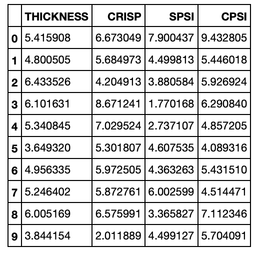
Something is still a little funny, all of our attribute scores should still be transformed to be between 0 and 10 as well. Let’s go ahead and do that. This time we’ll use the MinMaxScaler from Sklearn - MinMaxScaler does the same thing we did in the formula above to transform the pizza score!

I’m not transforming these scores for any reason other than a score of 1 to 10 seems to be the defacto scoring scale for pizza! Also, this will do something funny to our data that we’ll explore later.

scaler = MinMaxScaler()
pizza_features_df = scaler.fit_transform(pizza_features_df) * 10
pizza_features_df = pd.DataFrame(pizza_features_df, columns = pizza_attributes)
pizza_features_df.head(10)

Running the Regression

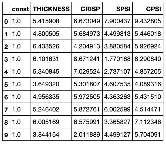
Next we’re going to run the regression itself. Before we do, we’re going to add the constant term to our dataframe. Recall our formula from above:

\(PizzaScore = B_0 + B_1 Thickness + B_2 Crisp + B_3 SPSI + B_4 CPSI + \epsilon\)

The term we’re adding to the dataframe is \(B_0\). Once we add the constant, our dataframe is going to look like this:

pizza_features_constant = sm.add_constant(pizza_features_df)
pizza_features_constant.head(10)

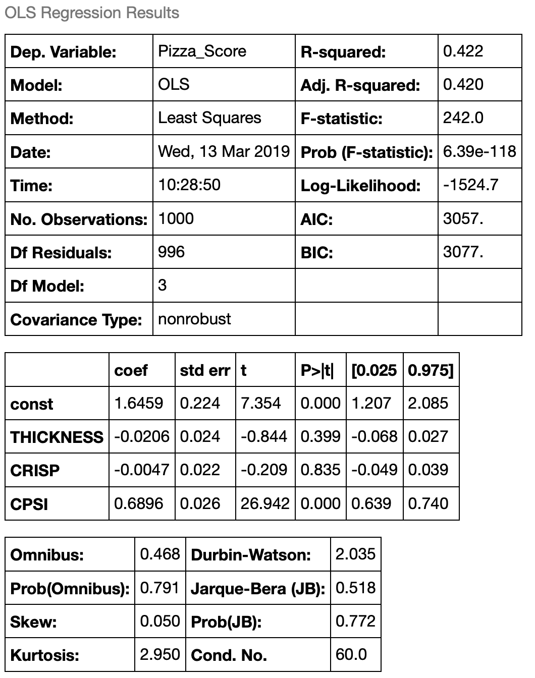
model = sm.OLS(pizza_score_df, pizza_features_constant)
lin_reg = model.fit() # Fit the regression line to the data
lin_reg.summary() # Output the summary of the regression

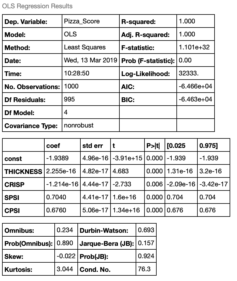
What do these results mean?

The output from the regressions spits out the above table. Let’s walk through these terms and talk about what they mean.

• R-squared: This is a value between 0 and 1 (also called the “coefficient of determination”) that tells us how much of the variation of the dependent variable (Pizza_Score) is described by our independent variables. We have a R-squared value of 1, which isn’t a surprise because we synthetically generated this data set to have 2 “informative variables” that describe the dependent variable. This means all of the variability of our pizza score is described by our independent variables.
• F-statistic: This is related to the R-squared value, and tells us how good the regression model is as a whole at describing the dependent variable.
• Prob(Omnibus): Is the probability that the errors from the dataset are normally distributed (an important assumption in regression models)
• Skew and Kurtosis: This tells you how “normally” distributed your data is. A normal distribution has a skew of 0.0 and kurtosis of 3.0. So we can see our data is very close to a normal distribution.
• Jarque-Bera and Prob (JB): The JB test is a test for normality. A very high value for JB is an indication that the data is likely not normally distributed. The Prob(JB) is the probability that the data is normally distributed based on the Jarque-Bera test. Note that this contrasts from Prob(Omnibus) which is a normality test on the errors, not the data points themselves.

Now scroll down a bit to where you see “coef”, “std err”, etc… The “coef” column is the beta coefficients for our equation. Observe that the coefficients for THICKNESS and CRISP are very small (zero). Also note that only two of the coefficients are non-zero. Namely, SPSI and CPSI. This is because when we generated our toy dataset we set the number of informative variables to be two. Our formula for our pizza score now becomes the following:

\(PizzaScore = -1.9389 + 0.704*SPSI + 0.676*CPSI + \epsilon\)

What this means is that for the individual in question - which is represented by the random pizza score dataset we created - the rating this person would apply to a pizza would abide by this formula.

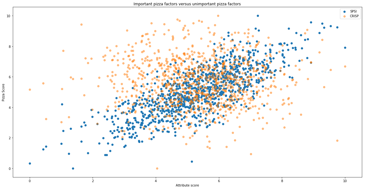
Visualizing the Important Pizza Factors

By plotting an important factor and an unimportant factor against pizza score, we can visually see the correlations. Here we plot SPSI (an important factor), and CRISP (an unimportant factor).

plt.figure(figsize=(20,10))
plt.scatter(pizza_score_df['Pizza_Score'],pizza_features_df['SPSI'])
plt.scatter(pizza_score_df['Pizza_Score'],pizza_features_df['CRISP'],alpha=0.5)
plt.xlabel('Attribute score')
plt.ylabel('Pizza Score')
plt.title("Important pizza factors versus unimportant pizza factors")
plt.legend()
plt.show

Principles of Model Specification (and what happens when you “misspecify”)

There are some compelling philosophies on model specification, in general, that I think are much easier to grasp within the context of our pizza example. They are as follows:

• The model should be grounded in logic: We should be able to supply reasoning behind the choice of variables, and the reasoning should make sense. For example, the color of the pizza box is likely an unreasonable factor to include in our pizza regression, but perhaps the “fluffiness” of the crust should be. Note that model specification, and feature engineering in general, often relies on the imagination of the people building the model. If there is something you can think of that might affect a person’s pizza score, it’s worth testing if it makes sense! This is the essence of science - develop a hypothesis and then test it.
• The law of parsimony: This means that fewer, high impact variables are better than a lot of variables. Each variable within a regression should play an important and impactful role. In our regression, sauce per square inch and cheese per square inch are definitely important and impactful.
• Violations of the regression assumptions should be examined before accepting the model: We haven’t discussed them yet, but the presence of heterskedasticity, multicollinearity, and serial correlation can call into question the validity of the regression model. We’ll discuss these shortly!
• Model should be useful on “real world data”: It’s fine and good to examine and explore the strength of relationships within a sample of data - but in order to test our Pizza regression model we would want to test it on new pizzas to see if it has a reasonable ability to “predict” whether or not this individual is bound to like the pizza - based on the sauce per square inch and cheese per square inch. This applies to all other statistical models as well - the “out-of-sample” test is the gold standard in determining whether or not the model is valid.

Misspecifying a model

The concept of misspecification is relatively straightforward. In our example, our regression results told us (by design) that there are two key variables that fully describe the variability in this individuals pizza score. If we were to remove one of these variables from the regression, we would no longer be able to explain the full variability in the dependent variable. It would be like trying to fully describe the flavour of a wine using only “acidity” as a descriptor, or Netwon trying to full explain force using only mass. To fully explain certain real-world phenomenon, there is typically a minimum number of variables that one needs to use - anything less than that would be a “misspecification”. It’s up to the data scientist to discover what these variables are.

Let’s try this on our pizza data to see what happens to the regression results. Let’s remove the “sauce per square inch” score and see what happens…

misspecified_df = pizza_features_constant.drop(['SPSI'], axis=1)
misspecified_df.head(10) # Our dataframe now looks like the following:

model_misspec = sm.OLS(pizza_score_df, misspecified_df)
lin_reg2 = model_misspec.fit()
lin_reg2.summary()

Can you see what happened here? By removing SPSI, a key independent variable, we forced the regression to try and explain the pizza score using only CPSI. This resulted in a few negative changes:

• Our R-squared value dropped significantly to 0.42. This makes sense. Our new regression is only able to describe 42% of the variability in the pizza score now that sauce per square inch has been removes.
• Our F-statistics dropped by many orders of maginitude.
• The t-statistics on our coefficients dropped because our standard errors increased significantly.
• There has been another subtle change as well that we didn’t discuss in the first one. Our Durbin-Watson statistic, which tells us if the residuals in the regression are serially correlated, increased to 2.035.
• Our confidence that the error terms are normally distributed has fallen. Model misspecification can be a really difficult thing to identify. Imagine we had done this regression first? Would it be obvious that we had “ommitted” a variable?
  
  

Collinearity, heteroscedasticity, and serial correlation

We have mentioned these three terms several times in this tutorial. These are, collectively, the “trifecta of no-no’s” when it comes to regression. It took my a while to wrap my head around these three things - mostly because they’re often presented poorly and in an uncessarily academic way (Or maybe I’m just a dummy!). In any case, I hope I do a better job of explaining these things here.

Heteroscedasticity

The word “scedastic” refers to the “variance of errors”. Homo, like homogeneous, refers to things being “identical”, or “of the same kind”. Hetero, is the opposite.

Heteroscedasticity refers to the variance of errors being different. Homoscedasticity refers to the variance of errors being the same. To illustrate an example of this let’s do a thought experiment. Imagine you’re standing on a beach and you have a basket of tennis balls. You drop the first tennis ball directly in front of you feet. You then record on a sheet of paper how far you “think” the ball is from your feet (in inches).

You then throw the second ball a little farther than the first, and again record the estimated distance down on your sheet of paper. You repeat this until you have to throw the balls as far as you possibly can down the beach - each time estimating how far they are from your feet in inches.

To finish the experiment, you mark your feet in the sand and then measure the exact distance of each ball from where your feet were. Do you think the error in the estimate for the final ball will be the same as the error in the estimate of the first ball? Likely not - it’s easy to estimate distance when something is very close. It’s much harder (more prone to error) when it’s far away.

If you were to plot the difference between the estimated distance and actual distance for each ball, it would likely increase in magnitude as the balls get further away. This is heteroscedasticity.

The presence of heteroscedasticity can invalidate the results of a regression because it assumes the variance of the errors are constant. Make sense?

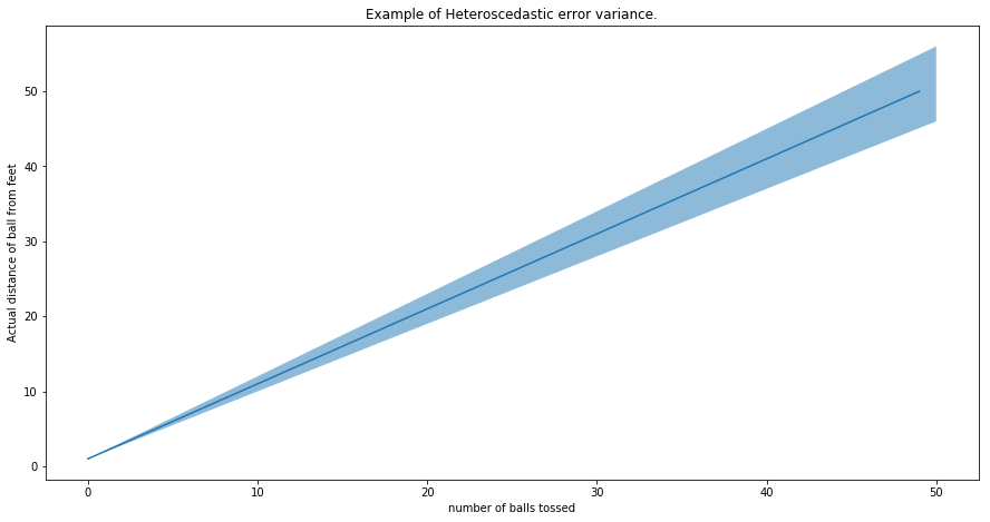
Below is a plot illustrating what heteroscedastic variance looks like visually. The shaded area, in this case, represents the potential error of our distance estimate. The solid red line is the actual estimate. With this plot we’re illustrating the example above - that estimating the distance of the ball from your feet will become harder the farther ball is away. The error variance, +/- 10% of the ball distance, has been chosen arbitrarily.

x=  np.linspace(1,50)
y = x
upper = 1+ 1.1 * x
lower = 1+ 0.90 * x
plt.figure(figsize = (15,7.5))
plt.plot(y)
plt.fill_between(x, upper, lower, alpha = 0.5)
plt.xlabel('number of balls tossed')
plt.ylabel('Actual distance of ball from feet')
plt.title("Example of Heteroscedastic error variance.")
plt.show()

Collinearity and Multicollinearity

This refers to the situation where any of the independent variables are significantly correlated with other independent variables.

For example, imagine in our pizza regression we introduced another sauce attribute called “Sauce volume”. We already have sauce per square inch as a scoring attribute. It makes sense that “sauce volume” and “sauce per square inch” are likely related. In fact, they might be perfectly correlated - or close to it. That is, if we increase sauce volume it has to go somewhere (spread around the pizza!).

Collinearity throws off regressions because when independent variables are correlated it can become impossible to determine how important each one is. Another word for collinearity is just “redundancy”. If you have two variables that move the same way, only one of them is required to explain the dependent variable - not both. To correct for collinearity, you just need to drop one of the variables. There are also libraries in python that can detect correlated variables and drop them automatically - although in most applications it’s important for the scientist to keep themselves in the loop.

Serial correlation (auto-correlation)

Serial correlation refers to the values of a timeseries being correlated with the a “lagged” version of itself. For example, if you boil a pot of water and leave it on the counter. Your best estimate for what the temperature is now is what the temperature was one period ago - in other words, the temperature of the pot from one second to the next aren’t random. Likewise, your best estimate for the temperature of the pot one second from now will be the temperature of the pot now, plus some error term.

In regression, one of the key assumptions is that the error terms (or residuals) are not serially correlated.

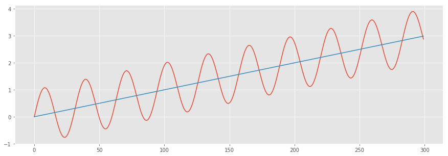
To visualize this, consider the sinusoid shown below with an upward sloping mean. If the mean is our “line of best fit” from the regression, the difference between the sinusoid and the mean line are the “residuals”. It’s clear that the residuals here aren’t random - they clearly follow the sinusoidal function. In this case, the residuals are “serially correlated”.

x = np.arange(300) # the points on the x axis for plotting

# compute the value (amplitude) of the sin wave at the for each sample
y = np.sin(0.2*x) + 0.01*x
z = 0.01*x

# showing the exact location of the smaples
plt.style.use('ggplot')
plt.figure(figsize=(15,5))
plt.plot(x,y,z)

Summary

• Regressions are used to find a linear combination of factors to describe a real-world phenomenon.
• Regression output in Python, and other sofware packages, tells you the following (at minimum):
  • The coefficient of determination (R-squared).
  • The regression coefficients and their corresponding standard errors and t-stats.
  • Skew and kurtosis of your data.
  • The probability that your data is normally distributed.
  • The probability that the residuals of your regression are normally distributed.
  • Whether or not the residuals are serially correlated.
  • The overall significance of the regression model (F-statistic).
• Heteroscedasticity is a term that means the variance of the errors in the regression is not constant. Although the presence of this does not affect the consistency of the regression estimators, it can cause the F-statistic to become unreliable.
• Multicollinearity is another term for “redundancy” with respect to the independent variables in a regression. If two of the independent variables are highly correlated, than determine the coefficients can be impossible and cause them to become unstable.
• Autocorrelation (or serial correlation) is a condition where data at one period is correlated to a lagged version of itself. In regressions, autocorrelation in the residuals can invalidate the results of the regression.
• In order for models to be properly specified:
  • The independent variables used should be grounded in logic.
  • The regression model should work on real world (out of sample) data.
  • The model should use the fewest high impact variables that is required to adequately describe the variance of the dependent variable.
  • None of the regression assumptions should be violated. The assumptions are:
    • There should be a linear relationship between the dependent variable and independent variables.
    • The independent variables are not random.
    • No exact linear relationship should exist between any of the independent variables.
    • The expected value of the error term should be 0. Meaning the error term is normally distributed.
    • The variance of the error term is the same for all observations (no heteroscedasticity)
    • The error term is no correlated across observations (no autocorrelation)

Thanks for reading!