Support Vector Machine Hyperparameter Tuning - A Visual Guide
Author :: Kevin Vecmanis
In this post I walk through the powerful Support Vector Machine (SVM) algorithm and use the analogy of sorting M&M’s to illustrate the effects of tuning SVM hyperparameters.
In this article you will learn:
- What s Support Vector Machine (SVM) is and what the main hyperparameters are
- How to plot the decision boundaries on simple data sets
- The effect of tuning degrees
- The effect of tuning C values
- The effect of using sigmoid, rbf, and poly kernels with SVM
Table of Contents
- Introduction
- The Effect of Changing the ‘Degree’ Parameter for Poly Kernel SVM
- The Effect of Using the RBF Kernel with different C Values
- The Effect of Using the Sigmoid Kernel with different C Values
- Summary
Introduction
In this post I’m going to repeat the experiment we did in our XGBoost post, but for Support Vector Machines - if you haven’t read that one I encourage you to view that first!
Support Vector Machines are one of my favourite machine learning algorithms because they’re elegant and intuitive (if explained in the right way). All this humble algorithm tries to do is draw a line in the dataset that seperates the classes with as little error as possible. Imagine you had a whole bunch of chocolate M&M’s on your counter top. Also, suppose that you only have two colors of M&M’s for this example: red and blue. A linear support vector machine would be equivalent to trying to seperate the M&M’s with a ruler (or some other straigh-edge device) in such a way that you get the best color seperation possible.
Using a poly support vector machine would be like using a ruler that you can bend and then use to seperate the M&M’s. A ‘1 degree poly’ support vector machine is equivalent to a straight line. Increasing the number of degrees allows you to have more bends in your ruler. You can imagine this might be handy depending on how mixed the pile of M&M’s is.
Using an rbf kernel support vector machine is for situations where you simply can’t use a straight ruler or bent ruler to effectively seperate the M&M’s. An analogy for RBF support vector machines would be where the M&M’s are so mixed that you have to ( if you could ) suspend the M&M’s in three dimensions and then try to seperate the two colors with a sheet of paper instead of a ruler (a hyperplane instead of a line).
During the demonstrations below, keep this analogy in mind. The datasets we show can be thought of as the M&M piles. There are three types of datasets and they’re designed to be seperated effectively by different types of support vector machines.
Below you’re going to see multiple lines and multiple color bands - this is because we’ve tasked the support vector machines to assign a probability of the datapoint being a blue dot or a red dot (Blue M&M or Red M&M). The different shades represent varying degrees of probability between 0 and 1.
The parameter C in each sub experiment just tells the support vector machine how many misclassifications are tolerable during the training process. C=1.0 represents no tolerance for errors. C=0.0 represents extreme tolerance for errors. In most real-world datasets, there can never be a perfect seperating boundary without overfitting the algorithm.
For a complete guide on SVM hyperparameters, visit the sklean page here: SVM Documentation
Let’s get started!
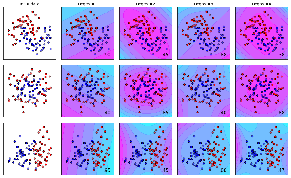
The Effect of Changing the Degree Parameter for Poly Kernel SVM
Note: We’re using the plot_decision_bounds function from the article on XGBoost Parameter Tuning
We can see visually from the results below what we talked about above - that the amount of “bend” in our ruler can determine how well we can seperate our pile of M&M’s.
- Degree 1 works best for dataset 1.
- Degree 4 works best for dataset 2.
- Degree 1 works best for dataset 3.
names = ['Degree=1', 'Degree=2', 'Degree=3', 'Degree=4']
classifiers = [SVC(probability=True, kernel='poly', degree=1, C=0.8),
               SVC(probability=True, kernel='poly', degree=2, C=0.8),
               SVC(probability=True, kernel='poly', degree=3, C=0.8),
               SVC(probability=True, kernel='poly', degree=4, C=0.8)]

plot_decision_bounds(names, classifiers)
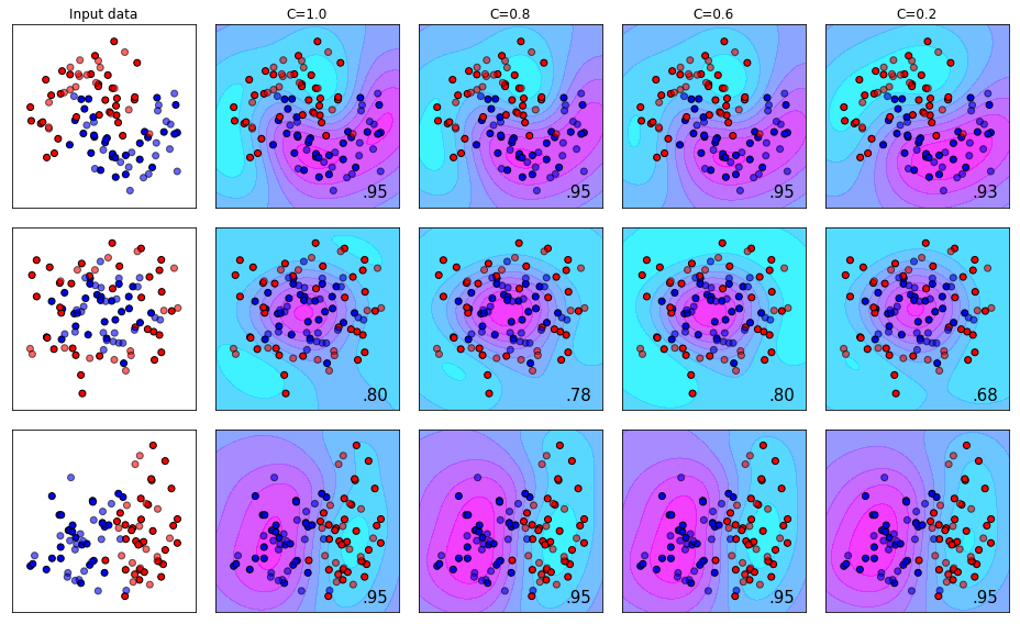
The Effect of Using the RBF Kernel with different C Values
Recall that the RBF kernel is suspending our pile of M&M’s in the air and trying to seperate them with a sheet of paper instead of using a ruler when they’re all flat on the counter top. The effect you see below is a 2-D projection of how the plane slices through the 3-D pile of M&M’s.
We can see here that the effect the C-value has is very much dependent on the dataset. This highlights the importance of visualizing your data at the beginning of a machine learning project so that you can see what you’re dealing with!
names = ['C=1.0', 'C=0.8', 'C=0.6', 'C=0.2']
classifiers = [SVC(probability=True, kernel='rbf', C=1.0),
               SVC(probability=True, kernel='rbf', C=0.8),
               SVC(probability=True, kernel='rbf', C=0.6),
               SVC(probability=True, kernel='rbf', C=0.2)]

plot_decision_bounds(names,classifiers)
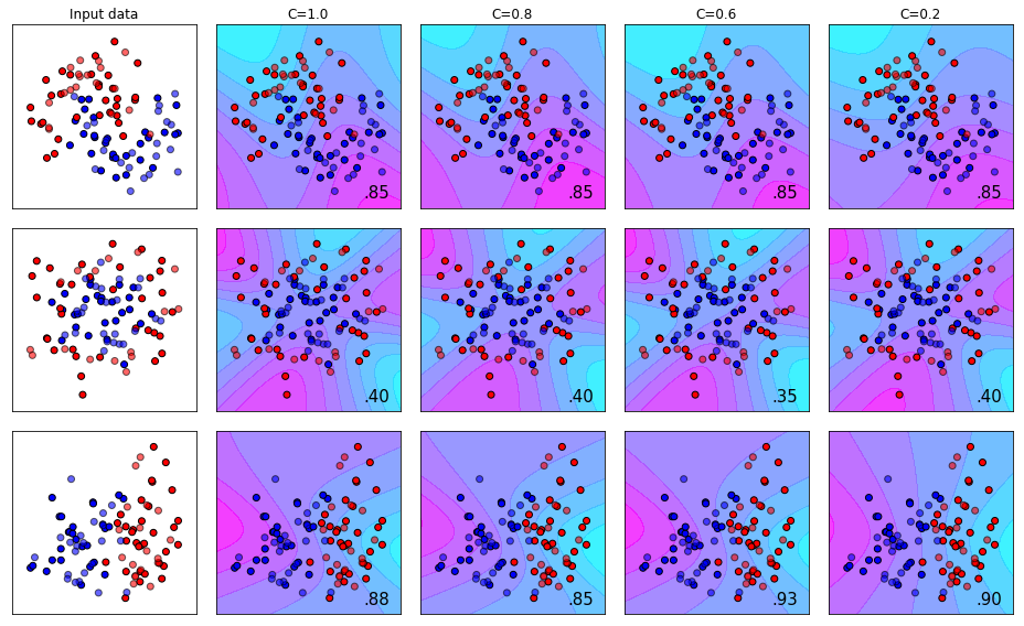
The Effect of Using the Sigmoid Kernel with different C Values
The sigmoid kernel is another type of kernel that allows more bend patterns to be used by the algorithm in the training process. The effect is visualized below.
names = ['C=1.0', 'C=0.8', 'C=0.6', 'C=0.2']
classifiers = [SVC(kernel='sigmoid',degree=3, C=1.0),
               SVC(kernel='sigmoid',degree=3, C=0.8),
               SVC(kernel='sigmoid',degree=3, C=0.6),
               SVC(kernel='sigmoid',degree=3, C=0.2)]

plot_decision_bounds(names,classifiers)
Summary
- Using M&M’s as an analogy, we can see that support vector machines attempt to seperate our pile of M&M’s as effectively as possible.
- Specifying the kernel type is akin to using different shaped rulers for seperating the M&M pile.
- The specific method that works best will be data-dependent.
- Support Vector Machines, to this day, are a top performing machine learning algorithm. The method it uses is intuitive if presented in the right way.
- One drawback of SVMs is that the computation time to train them scales quadratically with the size of the dataset. On large datasets the training time can be astronimical.
The top performers were:
- Dataset 1: RBF Kernel with C=1.0 (Score=0.95)
- Dataset 2: Poly Kernel with Degree=4 (Score=0.88)
- Dataset 3: Tie between Poly Kernel, Degree=1 and all four C-variants of the RBF Kernel (Score=0.95)
I hope you enjoyed this post!